R Implementation of marginal distributions
Description
The acc_margins function examines the impact of
so-called process variables on the measurement variables. This
implementation combines a descriptive and model-based approach.
acc_margins is an implementation of the Unexpected location and Unexpected proportion indicators, as
well as a descriptor for Unexpected
shape and Unexpected scale. These
belongs to the Unexpected
distributions domain in the Accuracy dimension.
For more details, see the user’s manual and source code.
Descriptive approach
For each level of the group_vars the marginal
distribution is shown in addition to an overall distribution. The
R-package ggplot2 is used to illustrate these distributions
in a combination of plot types. For:
- continuous data
and for
- discrete data
are used. The user is not obliged to specify whether measurements are
continuous or discrete. This is done by the acc_margins
function. Optional is the specification of the distribution in the
metadata.
Model-based approach
For the calculation of adjusted marginal means the R-package
emmeans is used which computes equally weighted marginal
effects of factor-variables. Details on the difference between crude
calculation of means and marginal effects is given in the very good
example provided by the emmeans package: Run
vignette("basics", package = "emmeans") to see the
corresponding vignette. emmeans can process a broad number
of different models
Lenth et al., 2016,, e.g. regression models with several
independent variables such as from multiple linear models or generalized
linear models. For each level of a process variable marginal
means are calculated including confidence intervals. The following
models are supported by this quality indicator function:
- linear models
- generalized linear models (binomial, 2 categories)
- generalized linear models (Poisson, \(\gt\) 2 categories but \(\le\) 15 categories)
Usage and arguments
acc_margins(
  resp_vars = NULL,
  group_vars = NULL,
  co_vars = NULL,
  label_col = "LABEL",
  threshold_value = 0.5,
  study_data = NULL,
  meta_data = NULL
)
The function has the following arguments:
- resp_vars: mandatory, a character specifying the measurement variable of interest. The variable must be of float or integer type.
- group_vars: the variable used for grouping (e.g.,
observer, device, reader). Defaults to
NULLfor output without grouping. - co_vars: optional, a vector of covariables, e.g. age or sex.
- threshold_type: optional, either empirical or user. In case empirical is chosen a multiplier of the scale measure is used, in case of user a value of the mean or probability (binary data) has to be defined see Implementation and use of thresholds
- threshold_value: a multiplier or absolute value. See also Implementation and use of thresholds.
- study_data: mandatory, the data frame containing the measurements.
- meta_data: mandatory, the data frame containing the item-level metadata.
- label_col: optional, the column in the metadata data frame containing the labels of all the variables in the study data.
We recommend specifying HARD_LIMITS
for the measurement variable (and for the covariables, if applicable) to
restrict the analysis to admissible numerical values. Similarly, VALUE_LABELS
for grouping variables ensure that only valid groups are considered
here.
Implementation and use of thresholds
The acc_margins function allows two different
specifications of thresholds using the same arguments of the
function.
Threshold: empirical
The specification of threshold_value is optional, since
the default of threshold_value is set to 1.
threshold_value serves as a multiplier of the following
measures:
- continuous data: standard deviation (SD)
- binary data: variance (\(p*(1-p)\))
- count data: variance (\(\lambda\))
Count data with more than 15 categories are treated as continuous data.
Threshold: user
If user is used instead, a threshold_value is a
mandatory argument. The meaning of threshold_value is
different to the threshold_type empirical. The
user may define a value on the measurement scale of the measurement
variable. For example, in case of SBP one may set
threshold_value to 120. Each level of the
aux_variable is highlighted if the confidence interval
of marginal means does not contain the predefined
threshold_value of 120. In case of a binomial distribution
the user must define the probability \(\in [0;
1]\).
This option should only be chosen if the distribution is known to the user.
Example output
To illustrate the output, we use the example synthetic data and metadata that are bundled with the dataquieR package. See the introductory tutorial for instructions on importing these files into R, as well as details on their structure and contents.
For the acc_margins function, the metadata columns
DATA_TYPE and MISSING_LIST are relevant:
| VAR_NAMES | LABEL | MISSING_LIST | DATA_TYPE | |
|---|---|---|---|---|
| 1 | v00000 | CENTER_0 | NA | integer |
| 3 | v00002 | SEX_0 | NA | integer |
| 4 | v00003 | AGE_0 | NA | integer |
| 6 | v01003 | AGE_1 | NA | integer |
| 7 | v01002 | SEX_1 | NA | integer |
| 8 | v10000 | PART_STUDY | NA | integer |
| 9 | v00004 | SBP_0 | 99980 | 99981 | 99982 | 99983 | 99984 | 99985 | 99986 | 99987 | 99988 | 99989 | 99990 | 99991 | 99992 | 99993 | 99994 | 99995 | float |
| 10 | v00005 | DBP_0 | 99980 | 99981 | 99982 | 99983 | 99984 | 99985 | 99986 | 99987 | 99988 | 99989 | 99990 | 99991 | 99992 | 99993 | 99994 | 99995 | float |
| 11 | v00006 | GLOBAL_HEALTH_VAS_0 | 99980 | 99983 | 99987 | 99988 | 99989 | 99990 | 99991 | 99992 | 99993 | 99994 | 99995 | float |
| 12 | v00007 | ASTHMA_0 | 99980 | 99988 | 99989 | 99991 | 99993 | 99994 | 99995 | integer |
| 14 | v00009 | ARM_CIRC_0 | 99980 | 99981 | 99982 | 99983 | 99984 | 99985 | 99986 | 99987 | 99988 | 99989 | 99990 | 99991 | 99992 | 99993 | 99994 | 99995 | float |
| 15 | v00109 | ARM_CIRC_DISC_0 | 99980 | 99981 | 99982 | 99983 | 99984 | 99985 | 99986 | 99987 | 99988 | 99989 | 99990 | 99991 | 99992 | 99993 | 99994 | 99995 | integer |
| 16 | v00010 | ARM_CUFF_0 | 99980 | 99987 | integer |
| 20 | v20000 | PART_PHYS_EXAM | NA | integer |
| 21 | v00014 | CRP_0 | 99980 | 99981 | 99982 | 99983 | 99984 | 99985 | 99986 | 99988 | 99989 | 99990 | 99991 | 99992 | 99994 | 99995 | float |
| 22 | v00015 | BSG_0 | 99980 | 99981 | 99982 | 99983 | 99984 | 99985 | 99986 | 99988 | 99989 | 99990 | 99991 | 99992 | 99994 | 99995 | float |
| 23 | v00016 | DEV_NO_0 | NA | integer |
| 25 | v30000 | PART_LAB | NA | integer |
| 26 | v00018 | EDUCATION_0 | 99980 | 99983 | 99988 | 99989 | 99990 | 99991 | 99993 | 99994 | 99995 | integer |
| 27 | v01018 | EDUCATION_1 | 99980 | 99983 | 99988 | 99989 | 99990 | 99991 | 99993 | 99994 | 99995 | integer |
| 28 | v00019 | FAM_STAT_0 | 99980 | 99983 | 99988 | 99989 | 99990 | 99991 | 99993 | 99994 | 99995 | integer |
| 29 | v00020 | MARRIED_0 | 99980 | 99983 | 99988 | 99989 | 99990 | 99991 | 99993 | 99994 | 99995 | integer |
| 30 | v00021 | N_CHILD_0 | 99980 | 99983 | 99988 | 99989 | 99990 | 99991 | 99993 | 99994 | 99995 | integer |
| 31 | v00022 | EATING_PREFS_0 | 99980 | 99983 | 99988 | 99989 | 99990 | 99991 | 99993 | 99994 | 99995 | integer |
| 32 | v00023 | MEAT_CONS_0 | 99980 | 99983 | 99988 | 99989 | 99990 | 99991 | 99993 | 99994 | 99995 | integer |
| 33 | v00024 | SMOKING_0 | 99980 | 99983 | 99988 | 99989 | 99990 | 99991 | 99993 | 99994 | 99995 | integer |
| 34 | v00025 | SMOKE_SHOP_0 | 99980 | 99983 | 99988 | 99989 | 99990 | 99991 | 99993 | 99994 | 99995 | integer |
| 35 | v00026 | N_INJURIES_0 | 99980 | 99983 | 99988 | 99989 | 99990 | 99991 | 99993 | 99994 | 99995 | integer |
| 36 | v00027 | N_BIRTH_0 | 99980 | 99983 | 99988 | 99989 | 99990 | 99991 | 99993 | 99994 | 99995 | integer |
| 37 | v00028 | INCOME_GROUP_0 | 99980 | 99983 | 99988 | 99989 | 99990 | 99991 | 99993 | 99994 | 99995 | integer |
| 38 | v00029 | PREGNANT_0 | 99980 | 99983 | 99988 | 99989 | 99990 | 99991 | 99993 | 99994 | 99995 | integer |
| 39 | v00030 | MEDICATION_0 | 99980 | 99983 | 99988 | 99989 | 99990 | 99991 | 99993 | 99994 | 99995 | integer |
| 40 | v00031 | N_ATC_CODES_0 | 99980 | 99983 | 99988 | 99989 | 99990 | 99991 | 99993 | 99994 | 99995 | integer |
| 43 | v40000 | PART_INTERVIEW | NA | integer |
| 44 | v00034 | ITEM_1_0 | 99980 | 99983 | 99988 | 99989 | 99991 | 99993 | 99994 | 99995 | integer |
| 45 | v00035 | ITEM_2_0 | 99980 | 99983 | 99988 | 99989 | 99991 | 99993 | 99994 | 99995 | integer |
| 46 | v00036 | ITEM_3_0 | 99980 | 99983 | 99988 | 99989 | 99991 | 99993 | 99994 | 99995 | integer |
| 47 | v00037 | ITEM_4_0 | 99980 | 99983 | 99988 | 99989 | 99991 | 99993 | 99994 | 99995 | integer |
| 48 | v00038 | ITEM_5_0 | 99980 | 99983 | 99988 | 99989 | 99991 | 99993 | 99994 | 99995 | integer |
| 49 | v00039 | ITEM_6_0 | 99980 | 99983 | 99988 | 99989 | 99991 | 99993 | 99994 | 99995 | integer |
| 50 | v00040 | ITEM_7_0 | 99980 | 99983 | 99988 | 99989 | 99991 | 99993 | 99994 | 99995 | integer |
| 51 | v00041 | ITEM_8_0 | 99980 | 99983 | 99988 | 99989 | 99991 | 99993 | 99994 | 99995 | integer |
| 53 | v50000 | PART_QUESTIONNAIRE | NA | integer |
We show two examples including different distributions of study data and assume that one examiner may not adhere to the SOP (Standard Operating Procedure). The following distributions are selected:
- continuous data
- count data with \(\le\) 15 categories
| v00000 | v00001 | v00002 | v00003 | v00004 | v00005 | v01003 | v01002 | v00103 | v00006 |
|---|---|---|---|---|---|---|---|---|---|
| 3 | LEIIX715 | 0 | 49 | 127 | 77 | 49 | 0 | 40-49 | 3.8 |
| 1 | QHNKM456 | 0 | 47 | 114 | 76 | 47 | 0 | 40-49 | 1.9 |
| 1 | HTAOB589 | 0 | 50 | 114 | 71 | 50 | 0 | 50-59 | 0.8 |
| 5 | HNHFV585 | 0 | 48 | 120 | 65 | 48 | 0 | 40-49 | 3.8 |
| 1 | UTDLS949 | 0 | 56 | 119 | 78 | 56 | 0 | 50-59 | 4.1 |
| 5 | YQFGE692 | 1 | 47 | 133 | 81 | 47 | 1 | 40-49 | 9.5 |
| 1 | AVAEH932 | 0 | 53 | 114 | 78 | 53 | 0 | 50-59 | 5.0 |
| 3 | QDOPT378 | 1 | 48 | 116 | 86 | 48 | 1 | 40-49 | 9.6 |
| 3 | BMOAK786 | 0 | 44 | 115 | 71 | 44 | 0 | 40-49 | 2.0 |
| 5 | ZDKNF462 | 0 | 50 | 116 | 74 | 50 | 0 | 50-59 | 2.4 |
margins_1 <- acc_margins(
  resp_vars = "SBP_0",
  group_vars = "USR_BP_0",
  co_vars = c("AGE_0", "SEX_0"),
  label_col = "LABEL",
  threshold_value = 0.5,
  study_data = sd1,
  meta_data = md1
)
The function generates two outputs: 1) A data frame (output 1)
summarizing the descriptive analysis results of emmeans
including a summary variable GRADING with 2 possible
values of 0 or 1, indicating whether data quality
issues were found. In the latter case (i.e, value = 1), one or more
levels of the group_variable deviates more than eligible from
the overall distribution (i.e., they are outside the threshold limits);
2) A summary plot (output 3) containing the marginal means including
confidence intervals. In case of oddities the marginal mean is displayed
in red.
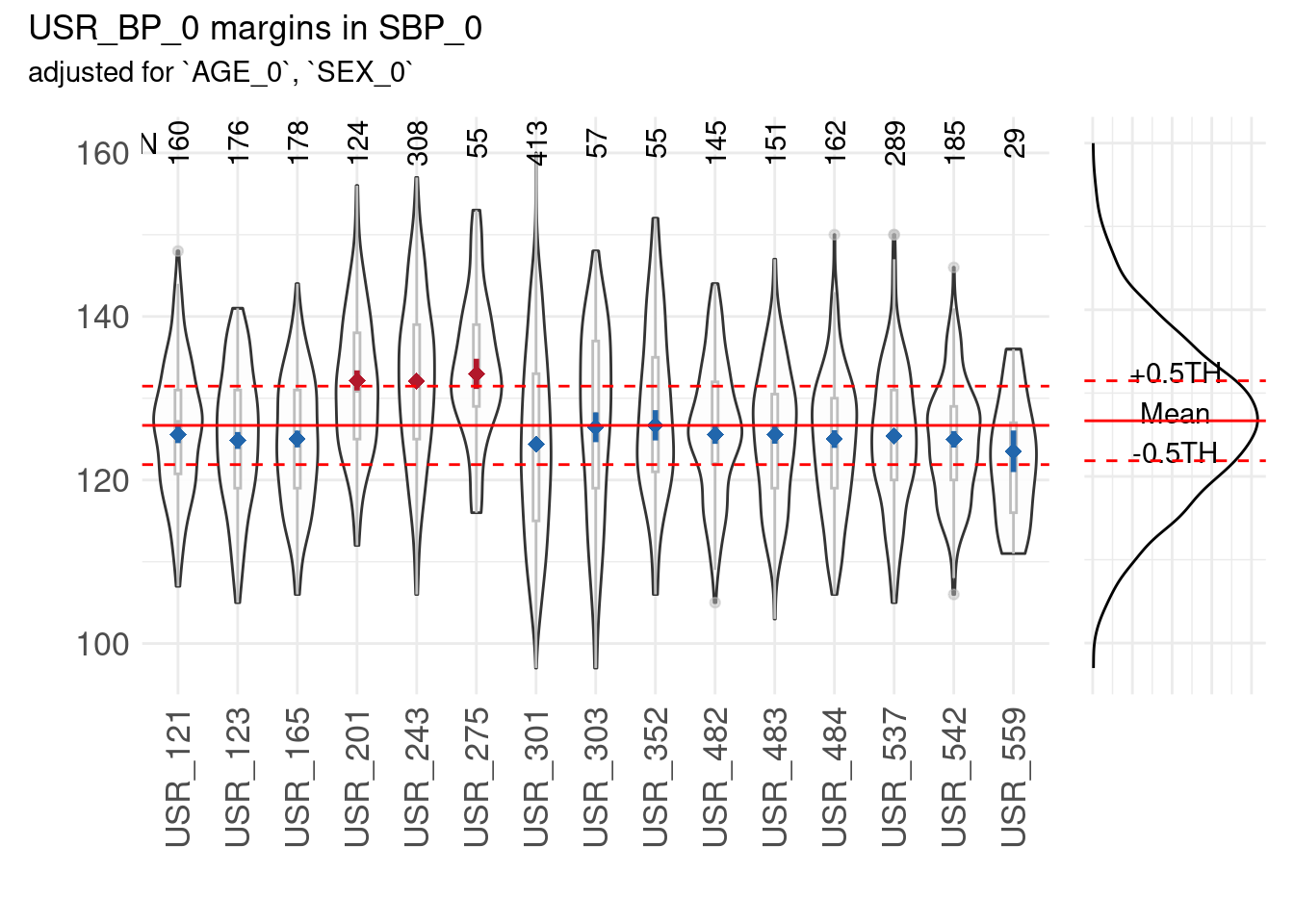
Example 1: normally distributed data
Output 1: Summary data frame for the different classes:
The summary data frame is called using
mp1$SummaryData:
| USR_BP_0 | margins | SE | n | CL |
|---|---|---|---|---|
| USR_121 | 125.5941 | 0.5526398 | 160 | [124.5104; 126.6778] |
| USR_123 | 124.8324 | 0.5267178 | 176 | [123.7995; 125.8653] |
| USR_165 | 125.0142 | 0.5236881 | 178 | [123.9873; 126.0412] |
| USR_201 | 132.1729 | 0.6283335 | 124 | [130.9407; 133.4050] |
| USR_243 | 132.0782 | 0.3980998 | 308 | [131.2975; 132.8588] |
| USR_275 | 132.9775 | 0.9420737 | 55 | [131.1301; 134.8248] |
| USR_301 | 124.3595 | 0.3437771 | 413 | [123.6853; 125.0336] |
| USR_303 | 126.4420 | 0.9256808 | 57 | [124.6269; 128.2572] |
| USR_352 | 126.6869 | 0.9435185 | 55 | [124.8367; 128.5370] |
| USR_482 | 125.5566 | 0.5805627 | 145 | [124.4181; 126.6950] |
| USR_483 | 125.5491 | 0.5685333 | 151 | [124.4343; 126.6640] |
| USR_484 | 125.0051 | 0.5489800 | 162 | [123.9286; 126.0816] |
| USR_537 | 125.4129 | 0.4110002 | 289 | [124.6069; 126.2188] |
| USR_542 | 124.9735 | 0.5137529 | 185 | [123.9661; 125.9809] |
| USR_559 | 123.5100 | 1.2977372 | 29 | [120.9652; 126.0547] |
Output 2: Summary Table
A table of summary data is generated for the respective variable.
This table provides the values of the calculated data quality
indicators, and it is necessary for the generic function
dataquieR::dq_report() to summarize all information for
examined variables.
| Variables | FLG_acc_ud_loc | PCT_acc_ud_loc |
|---|---|---|
| SBP_0 | 1 | 20 |
Output 3: Summary plot
The Summary plot is made of box plots and violin plots combined per level (e.g., per each examiner), and a density plot (flipped and aligned with the y-axis) on the right based on the overall data. The plots include lines of the overall mean and the deviation from the mean defined by the user via thresholds.
The summary plot frame is called using
mp1$SummaryPlot:
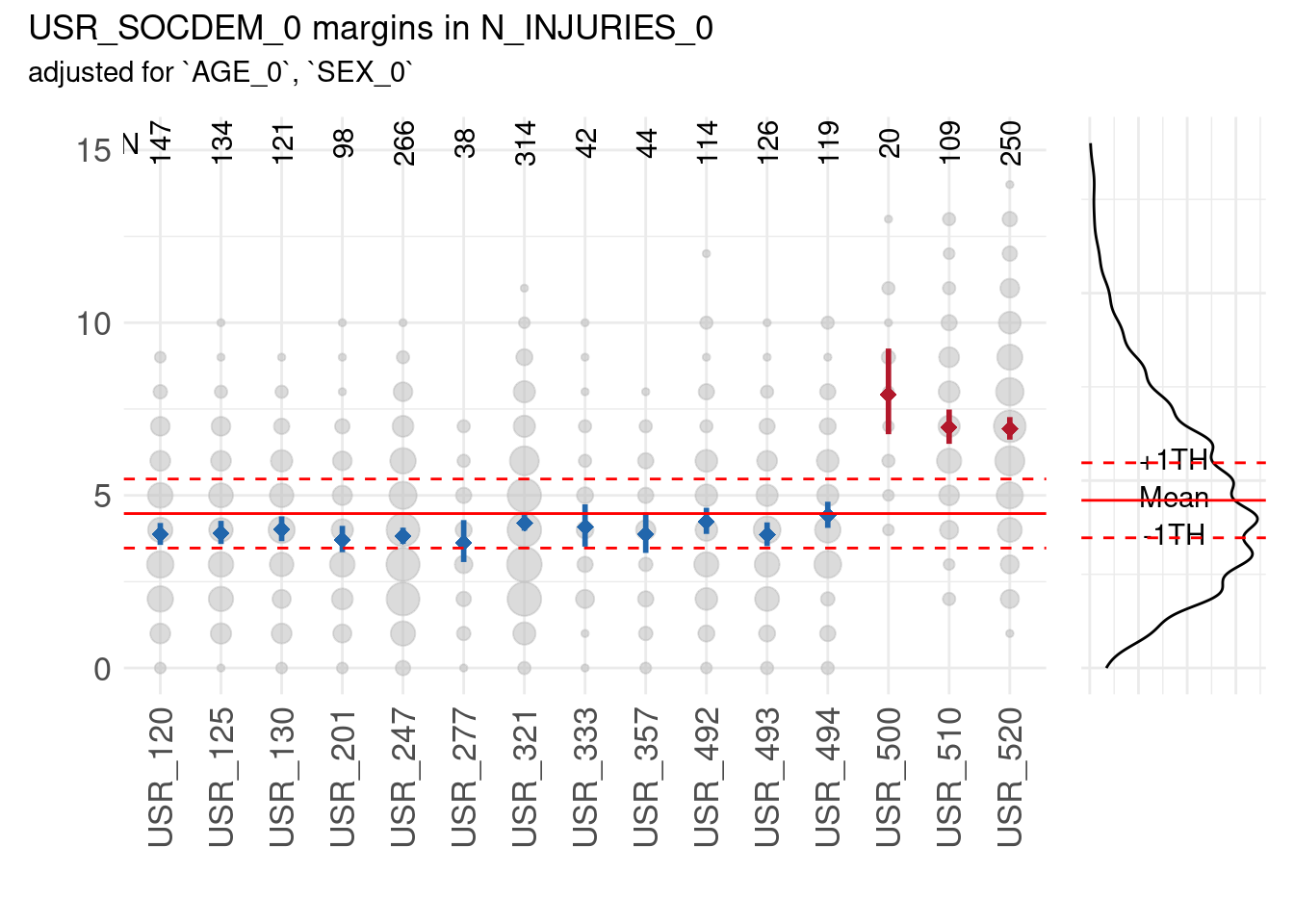
Example 2: count data
NOTE: If the number of categories exceeds 20 unique values the function will switch to a continuous distribution for the purpose of better illustration.
Output 3: Summary plot
The example regarding count data is restricted to the SummaryPlot
which can be called using margins_2$SummaryPlot:
Interpretation
Marginal means
Marginal means rests on model based results, i.e. a significantly different marginal mean depends on sample size. Particularly in large studies, small and irrelevant differences may become significant. The contrary holds if sample size is low.
Algorithm of the implementation
- The implementation can be applied on a single variable only.
- Missing codes are removed from
resp_vars(if defined in the metadata) - Deviations from limits, as defined in the metadata, are removed
- The distribution of
resp_varsis determined - The model-class fitting the distribution is selected (5a) The use of
co_varsfor adjustment is optional - An output data frame is generated for each level of
group_vars. - A summary plot is generated.
Limitations
Selecting the appropriate distribution is complex. Dozens of continuous, discrete or mixed distributions are conceivable in the context of epidemiological data. Their exact exploration is beyond the scope of this data quality approach. The function discriminates four cases:
- continuous data
- count data with \(\le\) 15 categories
- count data with \(\gt\) 15 categories
Nonetheless, only two different plot types are generated. The third case is treated as continuous data. This is in fact a coarsening of the original data but for the purpose of clarity this approach is chosen.
Concept relations
- Data quality Indicator Unexpected location
- Data quality Indicator Unexpected proportion
- Data quality Indicator Unexpected scale
- Data quality Indicator Unexpected shape
