Introductory Tutorial
This tutorial introduces the creation of data quality reports in R with dataquieR.
Loading data and metadata
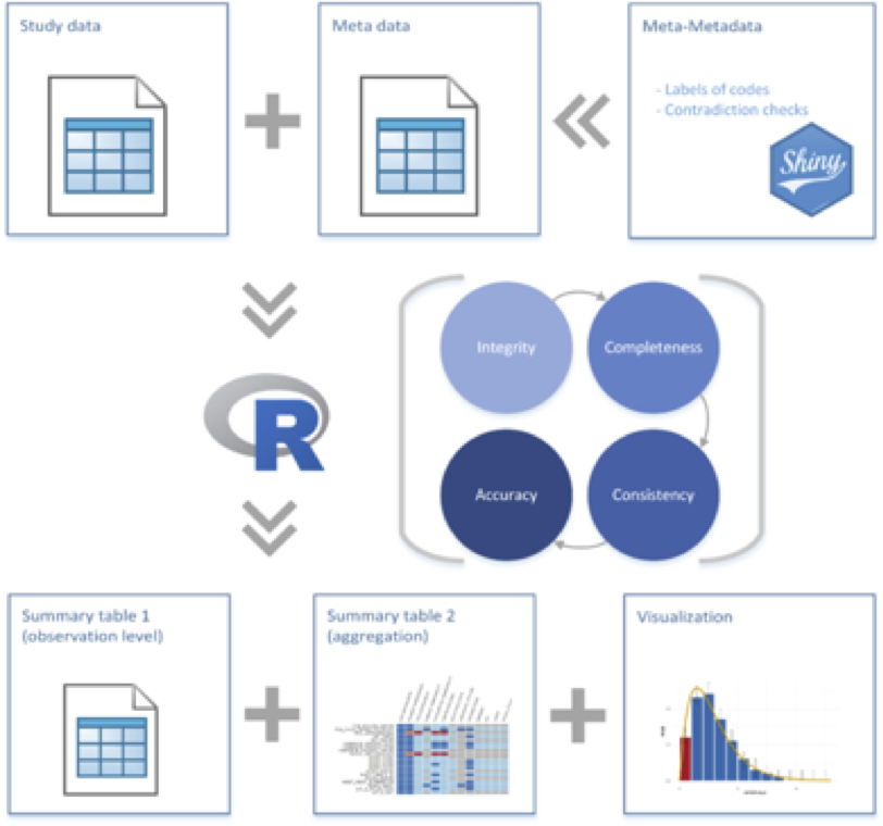
Creating reports requires the appropriate setup of study data and metadata, as shown in the figure below:

The first step is to
load dataquieR:
library(dataquieR)Then, we can load one of the example data sets using:
sd1 <- prep_get_data_frame("ship")This data set comes from the Study of Health in Pomerania (SHIP) project. The study data has 2154 observations and 33 variables:
sd1| id | exdate | age | sex | obs_bp | obs_soma | obs_int | dev_bp | dev_length | dev_weight |
|---|---|---|---|---|---|---|---|---|---|
| 3861 | 1998-09-22 | 65 | 1 | 9 | 9 | 11 | 18 | 11 | 11 |
| 6506 | 1998-01-21 | 70 | 1 | 4 | 4 | 3 | 9 | 3 | 1 |
| 6096 | 1999-04-07 | 43 | 2 | 4 | 4 | 2 | 10 | 3 | 1 |
| 6674 | 2000-10-06 | 55 | 2 | 3 | 5 | 2 | 22 | 4 | 1 |
| 6490 | 1998-11-17 | 69 | 2 | 7 | 7 | 12 | 18 | 11 | 11 |
| 5366 | 1997-11-27 | 65 | 1 | 5 | 5 | 1 | 10 | 3 | 1 |
| 5735 | 1999-09-01 | 40 | 2 | 7 | 7 | 23 | 15 | 11 | 11 |
| 4031 | 1999-08-12 | 51 | 2 | 9 | 9 | 12 | 20 | 11 | 11 |
| 3578 | 2000-02-26 | 25 | 1 | 9 | 9 | 22 | 15 | 11 | 11 |
| 4807 | 2000-07-13 | 80 | 2 | 3 | 3 | 2 | 18 | 4 | 1 |
We can see that not all variable names are intuitive. Hence, the appropriate labels must be mapped from the metadata. Besides all variables' data types and labels, the metadata stores further expected characteristics and static information about the study data.
We can load the corresponding example metadata using:
prep_load_workbook_like_file("ship_meta_v2")The metadata is a workbook containing several sheets or tables that can be called individually. The main metadata table is the item-level, which includes descriptions and expectations about single variables or items (e.g. columns in the study data table):
md1 <- prep_get_data_frame("item_level")| VAR_NAMES | LABEL | DATA_TYPE | SCALE_LEVEL | VALUE_LABELS | STANDARDIZED_VOCABULARY_TABLE | MISSING_LIST_TABLE | HARD_LIMITS |
|---|---|---|---|---|---|---|---|
| id | ID | integer | na | NA | NA | NA | NA |
| exdate | EXAM_DT_0 | datetime | interval | NA | NA | NA | [1995-01-01;) |
| sex | SEX_0 | integer | nominal | 1 = males | 2 = females | NA | NA | NA |
| age | AGE_0 | integer | ratio | NA | NA | NA | [20;Inf) |
| obs_bp | OBS_BP_0 | integer | nominal | 1 = Obs_01 | 2 = Obs_02 | 3 = Obs_03 | 4 = Obs_04 | 5 = Obs_05 | 6 = Obs_06 | 7 = Obs_07 | 8 = Obs_08 | 9 = Obs_09 | 10 = Obs_10 | 11 = Obs_11 | 12 = Obs_12 | 13 = Obs_13 | 14 = Obs_14 | 15 = Obs_15 | 16 = Obs_16 | 17 = Obs_17 | 18 = Obs_18 | 19 = Obs_19 | 20 = Obs_20 | NA | missing_table | NA |
| dev_bp | DEV_BP_0 | integer | nominal | 1 = Dev_01 | 2 = Dev_02 | 3 = Dev_03 | 4 = Dev_04 | 5 = Dev_05 | 6 = Dev_06 | 7 = Dev_07 | 8 = Dev_08 | 9 = Dev_09 | 10 = Dev_10 | 11 = Dev_11 | 12 = Dev_12 | 13 = Dev_13 | 14 = Dev_14 | 15 = Dev_15 | 16 = Dev_16 | 17 = Dev_17 | 18 = Dev_18 | 19 = Dev_19 | 20 = Dev_20 | 21 = Dev_21 | 22 = Dev_22 | 23 = Dev_23 | 24 = Dev_24 | 25 = Dev_25 | NA | missing_table | NA |
| sbp1 | SBP_0.1 | integer | ratio | NA | NA | NA | [80;200] |
| sbp2 | SBP_0.2 | integer | ratio | NA | NA | NA | [80;200] |
| dbp1 | DBP_0.1 | integer | ratio | NA | NA | NA | [40;160] |
| dbp2 | DBP_0.2 | integer | ratio | NA | NA | NA | [40;160] |
Additional details and expectations about the joint use of two or more variables or items are defined in the cross-item level metadata:
cil <- prep_get_data_frame("cross-item_level")| VARIABLE_LIST | CHECK_LABEL | CONTRADICTION_TERM | CONTRADICTION_TYPE | MULTIVARIATE_OUTLIER_CHECKTYPE | N_RULES | ASSOCIATION_RANGE | ASSOCIATION_METRIC |
|---|---|---|---|---|---|---|---|
| NA | Systolic blood pressure lower than dyastolic blood pressure, first measurement | [sbp1] < [dbp1] | LOGICAL | NA | NA | NA | NA |
| NA | Systolic blood pressure lower than dyastolic blood pressure, second measurement | [sbp2] < [dbp2] | LOGICAL | NA | NA | NA | NA |
| NA | Body height lower than body weight | [BODY_HEIGHT_0] < [BODY_WEIGHT_0] | LOGICAL | NA | NA | NA | NA |
| NA | Body height lower than waist circumference | [BODY_HEIGHT_0] < [WAIST_CIRC_0] | LOGICAL | NA | NA | NA | NA |
| NA | Contraception inconsistency | [SEX_0] = “males” and [CONTRACEPTIVA_EVER_0] = “yes” | LOGICAL | NA | NA | NA | NA |
| NA | Diabetes age inconsistency 1 | [DIABETES_KNOWN_0] = “yes” and [DIAB_AGE_ONSET_0] = “” | EMPIRICAL | NA | NA | NA | NA |
| NA | Diabetes age inconsistency 2 | [DIAB_AGE_ONSET_0] > 0 and not([DIABETES_KNOWN_0] = “yes”) | LOGICAL | NA | NA | NA | NA |
| sbp1 | sbp2 | Systolic blood pressure checks | NA | NA | Hubert | 1 | (0.7;) | Pearson |
| dbp1 | dbp2 | Diastolic blood pressure checks | NA | NA | Hubert | 1 | (0.7;) | Pearson |
| sbp1 | sbp2 | dbp1 | dbp2 | Blood pressure checks | NA | NA | NA | 4 | NA | NA |
Descriptions and expectations about the provided segments (e.g., different study examinations) are given in the segment level metadata:
sl <- prep_get_data_frame("segment_level")| STUDY_SEGMENT | SEGMENT_RECORD_COUNT | SEGMENT_ID_TABLE | SEGMENT_RECORD_CHECK | SEGMENT_ID_VARS | SEGMENT_UNIQUE_ROWS | SEGMENT_PART_VARS |
|---|---|---|---|---|---|---|
| INTRO | 2154 | expected_id_segment | exact | id | TRUE | seg_part_intro |
| SOMATOMETRY | 500 | expected_id_segment | exact | id | TRUE | seg_part_somatometry |
| INTERVIEW | 2150 | expected_id_segment | exact | id | TRUE | seg_part_interview |
| LABORATORY | 500 | expected_id_segment | subset | id | TRUE | seg_part_laboratory |
For more information on the example data and metadata, see the example data description and the metadata tutorial.
Generating a report
We can create a default report using the dq_report2()
function, which requires only the data and metadata previously
loaded:
dq_report2(study_data = sd1) # metadata will be found, if prep_load_workbook_like_file did run before.Minimal workflow example
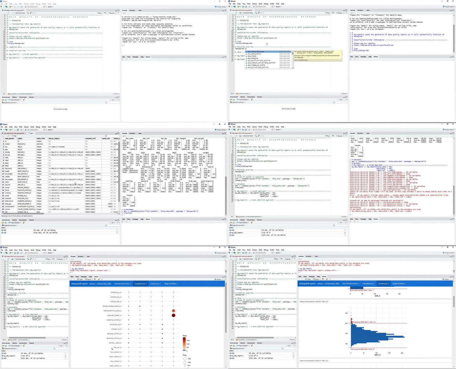
The animation below shows a quick workflow for reporting data quality with dataquieR:

r <- dq_report2("ship", meta_data_v2 = "ship_meta_v2")
dir.create("report_v2/")
print(r, dir = "report_v2/")
You can see the example report generated by dq_report2()
here.
Example code
The code shown in the animation to produce a report is given here:
# --------------------------------------------------------------------------------------------------
# D A T A    Q U A L I T Y   I N    E P I D E M I O L O G I C A L    R E S E A R C H
#
# == dataquieR
#
# dq_report2() eases the generation of data quality reports as it automatically calls dataquieR functions
#
#
# Installation/Further Information -----------------------------------------------------------------
#
# Please see our website:
# https://dataquality.qihs.uni-greifswald.de/
#
# (install dataquieR from CRAN using)
#
# or
#
# currently, you should install the development version as described
# on https://dataquality.ship-med.uni-greifswald.de/DownloadR.html

install.packages("dataquieR")


# load the package

library(dataquieR)

# data ---------------------------------------------------------------------------------------------

# Study of Health in Pomerania example data

sd1 <- prep_get_data_frame("ship")

print(sd1)

# metadata

prep_load_workbook_like_file("ship_meta_v2")

print(md1)

# dq_report2() - a crude approach -------------------------------------------------------------------

my_dq_report <- dq_report2(study_data = sd1,
                           meta_data_v2  = "ship_meta_v2",
                           label_col  = LABEL)

# view the results

print(my_dq_report)
The function dq_report2() and the print()
for such reports can manage further arguments and settings. However,
this sparse version is a good start to gaining insight into the data and
may serve as the base to tailor more specific reports.


