Creation of Simulated Data
Background
Within the DFG-project Standards and tools for the evaluation of data quality in complex epidemiological studies several implementations were developed to calculate different indicators of data quality. They address the data quality dimensions:
- integrity,
- completeness,
- consistency, and
- accuracy
of the data. To apply these R-functions in a reasonably sized data set the following simulated study data were created. In using simulated data, the true distortion is reproducible which is not guaranteed in real-world data. All methods to create the data and how distortion is introduced are annotated in this document.
The structure is as follows:
a clean set of study data is generated representing measurements of different examination types
reproducible distortion is introduced in the study data
In 3. and 4. a summary of the data is found.
1: Error-free data
The study data are fragmented into five different segments:
- ID variables
- Physical examination
- Laboratory
- Interview
- Questionnaire
Some of the segments define solitary examination areas while other comprise variables of global interest for conducting the study.
NOTE: None of the variables in the study data will
have self-explanatory names. The column names are technical which is
common in larger studies which manage their data in databases. Please
see the corresponding [Metadata] to find comprehensive variable names.
In the metadata a LABEL denotes these annotation:
ID variables
ID variables comprise a study center (integer) and a unique personal identifier.
set.seed(11235)
# Study center -------------------------------------------------------------------------------------
# Initialize data frame and add study center ID
df <- data.frame(v00000 = sample(1:5, 3000, replace = TRUE))
# PSEUDO-ID ----------------------------------------------------------------------------------------
# integer part
int <- data.frame(int_part = paste0(sample(0:9, size = 3000, replace = TRUE),
sample(0:9, size = 3000, replace = TRUE),
sample(0:9, size = 3000, replace = TRUE)))
# character part
int$ID <- NA
for (i in 1:dim(int)[1]) {
set.seed(i + 11235)
int$ID[i] <- paste0(paste0(LETTERS[sample(1:26, 5, replace = TRUE)],
collapse = ""), int$int_part[i])
}
# add pseudo-ID to df
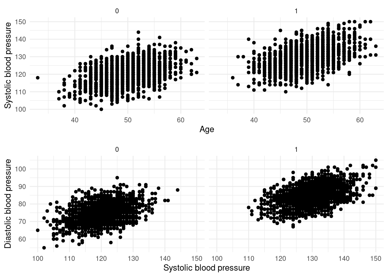
df$v00001 <- int$IDAge, sex and blood pressure
Age and sex are important covariates for the generation of blood pressure data. Therefore, age and sex-specific multivariate data of blood pressure are generated.
set.seed(11235)
# sex ----------------------------------------------------------------------------------------------
df$v00002 <- rbinom(n = 3000, size = 1, prob = 0.5)


# associated data of age and blood pressure --------------------------------------------------------
# mean age == 50, mean systolic blood pressure == 120/130, diastolic blood
# pressure 75/85
mu_male <- c(50, 130, 85)
mu_female <- c(50, 120, 75)

# definition of a covariance matrix which defines covariance structure
# (association)
Sigma <- matrix(c(20, 15, 12, 15, 45, 20, 12, 20, 35), 3, 3)

df$v00003 <- NA
df$v00004 <- NA
df$v00005 <- NA

# draw group specific multivariate normal data
df[df$v00002 == 0, c("v00003", "v00004", "v00005")] <-
  mvrnorm(n = table(df$v00002)[1], mu = mu_female, Sigma = Sigma)

# assign values for males
df[df$v00002 == 1, c("v00003", "v00004", "v00005")] <-
  mvrnorm(n = table(df$v00002)[2], mu = mu_male, Sigma = Sigma)

# round these data
df[, c("v00003", "v00004", "v00005")] <-
  dplyr::mutate_all(df[, c("v00003", "v00004", "v00005")],
    .funs = function(x) round(x, digits = 0))


# age and sex at follow-up -------------------------------------------------------------------------
df$v01003 <- df$v00003 + rbinom(3000, 1, prob = 0.01)
df$v01002 <- df$v00002


# Discretized age ----------------------------------------------------------------------------------
df$v00103 <- as.character(
  cut(df$v00003, breaks = c(18, 29, 39, 49, 59, 69, 100),
  labels = c("18-29", "30-39", "40-49", "50-59", "60-69", "70+")))
The data for age, systolic blood pressure and diastolic blood pressure are:
The simulated data show strong covariance between continuous measurement variables and a difference for sex.
Physical examination
In this segment of examination variables for:
- Asthma
- respiration capacity
- arm circumference
are generated. In addition, process variables are introduced as:
- examiners for blood pressure and respiratory examinations which are nested in each study center
- date variables of measurement
Please see Richter et al. for the role of process variables.
set.seed(11235)

# self reportet global health (VAS) ----------------------------------------------------------------
df$v00006 <- round(runif(3000, min = 0, max = 10), 1)


# RESPIRATION --------------------------------------------------------------------------------------
# Asthma
df$v00007  <- rbinom(3000, 1, prob = 0.2)

# high capacity in non-asthmatic participants
df$v00008 <- NA
df$v00008[df$v00007 == 0]  <- sample(LETTERS[1:5],
                                     length(df$v00008[df$v00007 == 0]),
                                     prob = seq(0.5, 0.05, length.out = 5),
                                     replace = TRUE)
# low capacity in asthmatic participants
df$v00008[df$v00007 == 1]  <- sample(LETTERS[1:5],
                                     length(df$v00008[df$v00007 == 1]),
                                     prob = seq(0.05, 0.5, length.out = 5),
                                     replace = TRUE)


# circumference upper arm --------------------------------------------------------------------------
df$v00009 <- round(rnorm(3000, mean = 25, sd = 4))
# discretize circumference
df$v00109 <- revalue(cut(df$v00009, breaks = c(-Inf, 20, 30, Inf)),
                     c("(-Inf,20]" = "1", "(20,30]" = "2", "(30, Inf]" = "3"))
df$v00109 <- as.integer(df$v00109)

# used arm cuff
df$v00010 <- revalue(cut(df$v00009, breaks = c(-Inf, 20, 30, Inf)),
                     c("(-Inf,20]" = "1", "(20,30]" = "2", "(30, Inf]" = "3"))

# Examiners respiration in each study center -------------------------------------------------------
df$v00011[df$v00000 == 1] <- sample(c("USR_101", "USR_103", "USR_155"),
                                    length(df$v00000[df$v00000 == 1]),
                                    replace = TRUE)
df$v00011[df$v00000 == 2] <- sample(c("USR_211", "USR_213", "USR_215"),
                                    length(df$v00000[df$v00000 == 2]),
                                    prob = c(0.4, 0.4, 0.2),
                                    replace = TRUE)
df$v00011[df$v00000 == 3] <- sample(c("USR_321", "USR_333", "USR_342"),
                                    length(df$v00000[df$v00000 == 3]),
                                    prob = c(0.8, 0.1, 0.1),
                                    replace = TRUE)
df$v00011[df$v00000 == 4] <- sample(c("USR_402", "USR_403", "USR_404"),
                                    length(df$v00000[df$v00000 == 4]),
                                    replace = TRUE)
df$v00011[df$v00000 == 5] <- sample(c("USR_590", "USR_592", "USR_599"),
                                    length(df$v00000[df$v00000 == 5]),
                                    prob = c(0.6, 0.35, 0.05),
                                    replace = TRUE)

# Examiner blood pressure in each study center -----------------------------------------------------
df$v00012[df$v00000 == 1] <- sample(c("USR_121", "USR_123", "USR_165"),
                                    length(df$v00000[df$v00000 == 1]),
                                    replace = TRUE)
df$v00012[df$v00000 == 2] <- sample(c("USR_201", "USR_243", "USR_275"),
                                    length(df$v00000[df$v00000 == 2]),
                                    prob = c(0.25, 0.65, 0.1),
                                    replace = TRUE)
df$v00012[df$v00000 == 3] <- sample(c("USR_301", "USR_303", "USR_352"),
                                    length(df$v00000[df$v00000 == 3]),
                                    prob = c(0.8, 0.1, 0.1),
                                    replace = TRUE)
df$v00012[df$v00000 == 4] <- sample(c("USR_482", "USR_483", "USR_484"),
                                    length(df$v00000[df$v00000 == 4]),
                                    replace = TRUE)
df$v00012[df$v00000 == 5] <- sample(c("USR_537", "USR_542", "USR_559"),
                                    length(df$v00000[df$v00000 == 5]),
                                    prob = c(0.6, 0.35, 0.05),
                                    replace = TRUE)


# Date-Time of examination -------------------------------------------------------------------------
dates   <- as.POSIXct(seq(0, 364, length = 3000) * 3600 * 24, origin =
                        as.Date("2018-12-31") - 364)
wd      <- weekdays(dates, abbreviate = TRUE)
wddates <- sample(dates[wd %in% c("Mon", "Tue", "Wed", "Thu", "Fri")], 3000,
                  replace = TRUE)

df$v00013 <- wddates[order(wddates)]
Laboratory
In this segment variables for:
- c-reactive protein (CRP)
- erythrocyte sedimentation rate (ESR)
as well as for process variables of:
- a measurement device
- and the date of measurement
are generated.
set.seed(11235)

# CRP ----------------------------------------------------------------------------------------------
df$v00014 <- round(rgamma(3000, shape = 3, scale = 1), digits = 3)

# ESR ----------------------------------------------------------------------------------------------
df$v00015 <- round(rgamma(3000, shape = 1.5, scale = 1) * 10, digits = 0)

# Lab device number --------------------------------------------------------------------------------
df$v00016 <- sample(1:5, 3000, replace = TRUE)


# Date-Time of Lab ---------------------------------------------------------------------------------
# on average 2 hours after exam date
df$v00017 <- df$v00013 + minutes(round(rnorm(3000, mean = 120, sd = 10),
                                       digits = 0))
Interview
Very typical in epidemiological studies is the a high number of information originating from interviews. The following variables are generated here:
- education
- family status
- number of children
- eating preferences
- smoking habits
- number of injuries
- number of birth
- pregnancies
- groups of income
- use of medication
- ATC-codes for used medication
as well as an examiner and a date variable for the conduct of the interview.
set.seed(11235)
# education ----------------------------------------------------------------------------------------
# baseline
df$v00018 <- rtpois(3000, 3, a = -1, b = 6)

# follow-up (some achieve higher qualification)
df$v01018 <- df$v00018 + rbinom(3000, 1, prob = 0.01)

# Family status ------------------------------------------------------------------------------------
df$v00019 <- sample(0:3, size = 3000, prob = c(0.25, 0.35, 0.3, 0.1), replace = TRUE)
df$v00020 <- ifelse(df$v00018 == 1, 1, 0)


# No. of children ----------------------------------------------------------------------------------
df$v00021 <- rpois(3000, lambda = 2.5)

# eating behaviour ---------------------------------------------------------------------------------
# (no preference, vegetarian, vegan)
df$v00022 <- sample(0:2, 3000, prob = c(0.6, 0.3, 0.1), replace = TRUE)

# vegetarian/vegan -> no meat consumption
df$v00023[df$v00022 > 0] <- 0
# no preferences -> frequency of shopping meat
df$v00023[df$v00022 == 0] <- sample(0:4,
                                    length(df$v00022[df$v00022 == 0]),
                                    prob = c(0.05, 0.25, 0.3, 0.2, 0.1),
                                    replace = TRUE)

# smoking habbits ----------------------------------------------------------------------------------
df$v00024 <- rbinom(3000, 1, prob = 0.3)        # current smoking
df$v00025 <- sample(0:4, 3000, replace = TRUE)  # shopping tabacco
# non-smokers conditional missing in tobacco shopping
df$v00025[df$v00024 == 0] <- NA


# No. of injuries ----------------------------------------------------------------------------------
df$v00026 <- rpois(3000, lambda = 4)

# No. of birth -------------------------------------------------------------------------------------
df$v00027 <- df$v00021 + rpois(3000, lambda = 1)

# no birth in men (jump code)
df$v00027[df$v00002 == 1] <- 88880

# Groups of income ---------------------------------------------------------------------------------
df$v00028 <- rtpois(3000, 2, a = -1, b = 5)


# pregnancy ----------------------------------------------------------------------------------------
df$v00029 <- rbinom(1000, 1, prob = 0.05)

# no pregnant men (jump code)
df$v00029[df$v00002 == 1] <- 88880

# some medication ----------------------------------------------------------------------------------
df$v00030 <- sample(c(NA, 1, 2, 3), 1000, prob = c(0.7, 0.1, 0.1, 0.1), replace=TRUE)

# ATC-Codes ----------------------------------------------------------------------------------------
df$v00031 <- rnbinom(3000, 1, prob = 0.3)


# Examiner soc.-demogr. ----------------------------------------------------------------------------
df$v00032[df$v00000 == 1] <- sample(c("USR_120", "USR_125", "USR_130"),
                                    length(df$v00000[df$v00000 == 1]),
                                    replace = TRUE)
df$v00032[df$v00000 == 2] <- sample(c("USR_201", "USR_247", "USR_277"),
                                    length(df$v00000[df$v00000 == 2]),
                                    prob = c(0.25, 0.65, 0.1),
                                    replace = TRUE)
df$v00032[df$v00000 == 3] <- sample(c("USR_321", "USR_333", "USR_357"),
                                    length(df$v00000[df$v00000 == 3]),
                                    prob = c(0.8, 0.1, 0.1),
                                    replace = TRUE)
df$v00032[df$v00000 == 4] <- sample(c("USR_492", "USR_493", "USR_494"),
                                    length(df$v00000[df$v00000 == 4]),
                                    replace = TRUE)
df$v00032[df$v00000 == 5] <- sample(c("USR_500", "USR_510", "USR_520"),
                                    length(df$v00000[df$v00000 == 5]),
                                    prob = c(0.05, 0.35, 0.6),
                                    replace = TRUE)

# Date-Time of Interview ---------------------------------------------------------------------------
# on average 30 minutes after lab date
df$v00033 <- df$v00017 + minutes(round(rnorm(3000, mean = 30, sd = 7),
                                       digits = 0))
The corresponding data are stored as integer, string, and datetime variables.
Questionnaire
The questionnaire contains an 8-item scale instrument measuring on a numeric rating scale (0-10). In addition, a corresponding date is generated.
set.seed(11235)

# 8-item questionnaire -----------------------------------------------------------------------------
# comment: rtpois() is different to rpois() since the distribution can be truncated
# first 4 items having "mean" 3
part1 <- data.frame(matrix(rtpois(12000, 3, a = -1, b = 10), ncol = 4))
# second 4 items having "mean" 7
part2 <- data.frame(matrix(rtpois(12000, 7, a = -1, b = 10), ncol = 4))

quest <- data.frame(part1, part2)
colnames(quest) <- c("v00034", "v00035", "v00036", "v00037",
                     "v00038", "v00039", "v00040", "v00041")

df <- cbind(df, quest)

# Date-Time of Questionnaire -----------------------------------------------------------------------
# on average 14 days after exam date
df$v00042 <- df$v00013 + days(round(rnorm(3000, mean = 14, sd = 3), digits = 0))
The data are:
2: Introduce distortion
Although data quality indicators should be applied in the sequence of (1) completeness, (2) consistency and then (3) accuracy the distortion to the data is added in a different sequence. Completeness affects all variables and is introduced here last.
The errors introduced into the study data are explained step by step along with the data quality dimensions. Some of these errors are specific to random subsets of the study data as defined here:
set.seed(11235)
ns <- 1:3000

# a 10pct sample (disjunct from 5 pct sample)
sam10  <- sample(ns, 300, replace = FALSE)
# a 5pct sample
sam5   <- sample(ns[!(ns %in% sam10)], 150, replace = FALSE)
Consistency
- Age during follow-up, some become younger than at baseline
# age and sex at follow-up -----------------------------------------------------
df$v01003[sam5] <- df$v00003[sam5] - 1- some participants switch sex between baseline and follow-up
df$v01002[sam5] <- abs(df$v00002[sam5] - 1)The arm cirmumference is important to choose the appropriate arm cuff for blood pressure measurement.
- in some the false arm-cuff (size) is used
# used cuff --------------------------------------------------------------------
# discretize arm circumference and add some failure of the assignment of the
# used cuff
df$v00010 <- revalue(cut(df$v00009 + round(rnorm(3000)),
                         breaks = c(-Inf, 20, 30, Inf)),
                     c("(-Inf,20]" = "1", "(20,30]" = "2", "(30, Inf]" = "3"))
df$v00010 <- as.integer(df$v00010)- some participants mention a lower level of education at follow up
# education --------------------------------------------------------------------
df$v01018[sam5][df$v01018[sam5] > 0] <- df$v01018[sam5][df$v01018[sam5] > 0] +
  rbinom(length(df$v01018[sam5][df$v01018[sam5] > 0]),
1, prob = 0.1) * -1- some vegetarian + vegan consume meat
# eating behaviour -------------------------------------------------------------
df$v00023[sam10][df$v00022[sam10] > 0] <- sample(1:4,
                                               length(df$v00023[sam10][
                                                 df$v00022[sam10] > 0]),
replace = TRUE)- some non-smokers shop tobacco
# smoking habbits --------------------------------------------------------------
df$v00025[sam10][is.na(df$v00025[sam10])] <- sample(1:5,
                                                    length(df$v00025[sam10][
                                                      is.na(df$v00025[sam10])]),
                                                    replace = TRUE)
Within the questionnaire the direction of questions differ between the first four items and the last 4 items. It is expected that the mean of answers changes accordingly. However,
- some participants answer monotonously
# 8-item questionnaire ---------------------------------------------------------
# some didn't recognize changed coding (numbers are usually from poisson with
# lambda = 7)
df$v00038[c(sam5, sam10)] <- rtpois(length(df$v00038[c(sam5, sam10)]), 3,
                                    a = -1, b = 10)
df$v00039[c(sam5, sam10)] <- rtpois(length(df$v00039[c(sam5, sam10)]), 3,
                                    a = -1, b = 10)
df$v00040[c(sam5, sam10)] <- rtpois(length(df$v00040[c(sam5, sam10)]), 3,
                                    a = -1, b = 10)
df$v00041[c(sam5, sam10)] <- rtpois(length(df$v00041[c(sam5, sam10)]), 3,
                                    a = -1, b = 10)
The study protocol foresees a sequence of examinations. Therefore, datetimes of study segments are expected in a predefined sequence.
- in some participants laboratory examination is done prior physical examination
- some questionnaires are returned very late and some very early
# Date variables ---------------------------------------------------------------
# lab earlier than physical examination
df$v00017[sam10] <- df$v00017[sam10] - hours(2)

# some late questionnaire
df$v00042[sam5] <- df$v00042[sam5] + days(sample(15:730, length(sam5),
                                                 replace = TRUE))

# some early questionnaire
df$v00042[sample(sam10, 10)] <- "2017-12-31 23:59:59"
Accuracy
- rounding of blood pressure measurements is done by some examinares. Please see the consequences at the bottom of this section.
set.seed(11235)

# Blood pressure: ----------------------------------------------------------------------------------
# rounding values to 80 (SBP) and 70 (DBP)
# in Cologne severe rounding at carneval
df$v00004[df$v00000 == 4 & month(df$v00013) == 2] <- plyr::round_any(df$v00004[
  df$v00000 == 4 & month(df$v00013) == 2], 10)
df$v00005[df$v00000 == 4 & month(df$v00013) == 2] <- plyr::round_any(df$v00005[
df$v00000 == 4 & month(df$v00013) == 2], 10)- one laboratory device generates large amounts of data at the detection limit of CRP
# Accumulation of values on detection limits -----------------------------------
# CRP: one device all values on detection limit (Oct-Dec)
df$v00014[df$v00016 == "1" & month(df$v00013) %in% 10:12] <- 0.16- some values of ESR are rounded by some examiners
# Some values of ESR were rounded ----------------------------------------------
df$v00015[c(sam5, sam10)] <- plyr::round_any(df$v00015[c(sam5, sam10)], 10)- one device is more often used than others
# One device is more often used ------------------------------------------------
df$v00016[month(df$v00013) %in% 1:3] <- sample(1:3,
                                               length(df$v00016[month(df$v00013)
                                                                %in% 1:3]),
replace = TRUE)- in one study center the reporting of used medication differs to other study centers
# Participants report a lower number of used drugs in one center  --------------
df$v00031[df$v00000 == 1 & df$v00031 > 3] <- df$v00031[df$v00000 == 1 &
                                                         df$v00031 > 3] -
ceiling(0.5 * df$v00031[df$v00000 == 1 & df$v00031 > 3])- one interviewer animates participants to report higher numbers of injuries
# Participants report a higher number of injuries if asked by one examiner -----
df$v00026[df$v00000 == 5] <- df$v00026[df$v00000 == 5] + sample(1:5,
                                                                length(
                                                                  df$v00026[
                                                                    df$v00000 ==
                                                                      5]),
replace = TRUE)- SBP/DBP follow linear trend in one study center
l_trend <- seq(15, 0, length.out = table(df$v00000)[2])

df$v00004[df$v00000 == 2] <- df$v00004[df$v00000 == 2] +
  round(l_trend, digits = 0)
df$v00005[df$v00000 == 2] <- df$v00005[df$v00000 == 2] +
round(l_trend, digits = 0)- SBP/DBP follow sigmoidal trend in another study center
s_trend <- sin(seq(0, 6.282, length = table(df$v00000)[3])) * 10

df$v00004[df$v00000 == 3] <- df$v00004[df$v00000 == 3] + round(s_trend,
                                                               digits = 0)
df$v00005[df$v00000 == 3] <- df$v00005[df$v00000 == 3] + round(s_trend,
                                                               digits = 0)

# seasonal abuse of medics 2018-09-22 - 2018-10-07 -----------------------------
df$v00030[df$v00033 >= "2018-09-22" & df$v00033 <= "2018-10-08"] <- 1
ggplot(df, aes(x = v00013, y = v00004)) + geom_point(aes(color = v00000)) +
facet_grid(v00000 ~ .) +
theme_minimal() +
theme(legend.position = "None")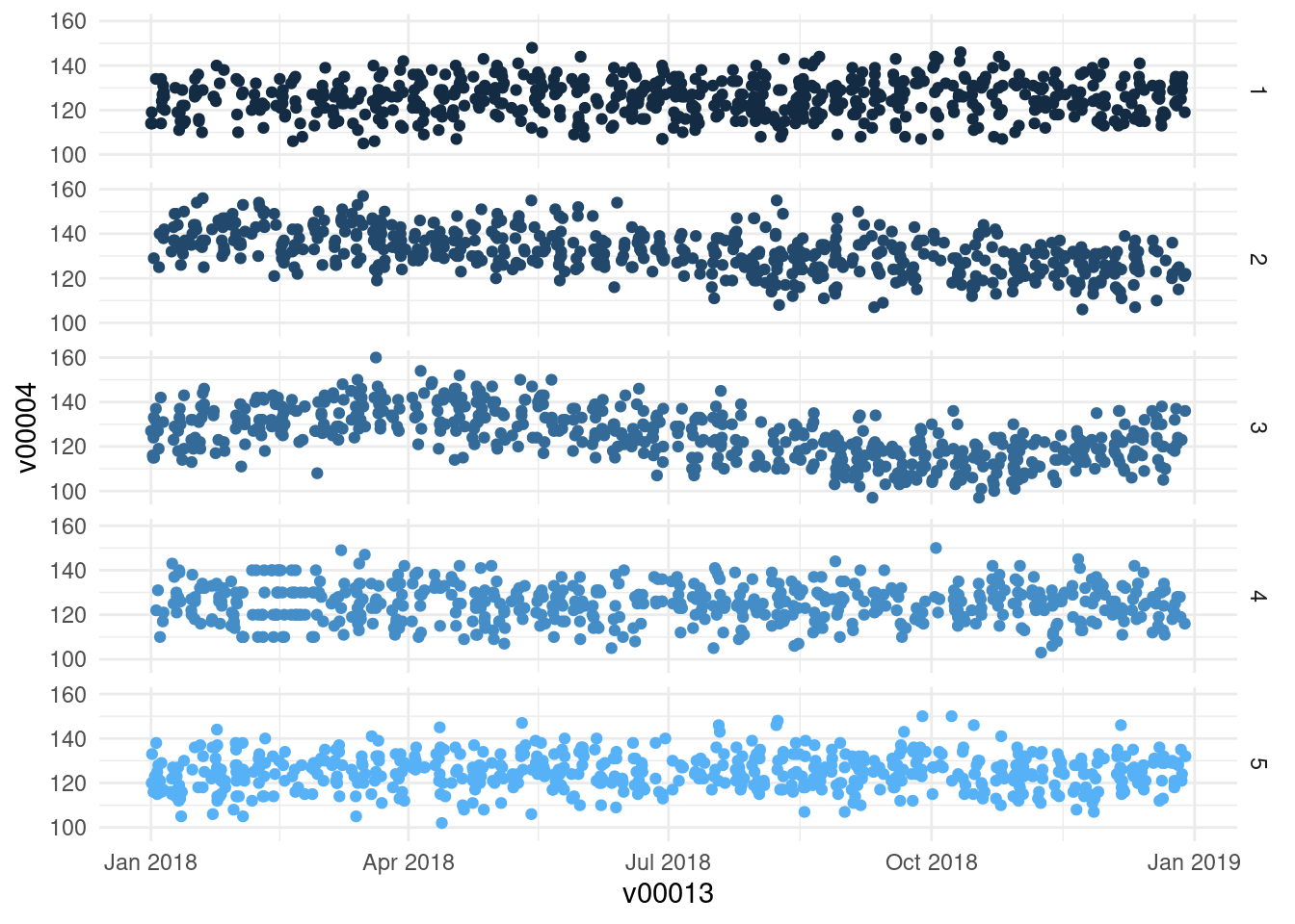
ggplot(df, aes(x = v00013, y = v00005)) + geom_point(aes(color = v00000)) +
  facet_grid(v00000 ~ .) +
  theme_minimal() +
  theme(legend.position = "None")
Completeness
Item missingness
Missing values in measurement variables can be informative, i.e. the reason for missingness is known, or uninformative. The latter is usually indicated by NAs. However, for the investigation of data quality and for examination of possible means of intervention (in the data generating process) the knowledge of reasons for missingness is crucial. The following code introduces both types of missingness.
Therefore, missing codes from the metadata were collected:
set.seed(11235)

#-------------------------------------------------------------------------------
# missing codes physical exam and lab
codesPL <- list( c(99980, 99981, 99982, 99983, 99984, 99985, 99986, 99987,
                   99988,
                   99989, 99990, 99991, 99992, 99993, 99994, 99995),
                 c(99980, 99981, 99982, 99983, 99984, 99985, 99986, 99987,
                   99988,
                   99989, 99990, 99991, 99992, 99993, 99994, 99995),
                 c(99980, 99983,  99987, 99988, 99989, 99990, 99991, 99992,
                   99993,
                   99994, 99995),
                 c(99980,  99988, 99989, 99991, 99993, 99994, 99995),
                 c(99980, 99983,  99987, 99988, 99989, 99990, 99991, 99992,
                   99993,
                   99994, 99995),
                 c(99980, 99981, 99982, 99983, 99984, 99985, 99986, 99987,
                   99988,
                   99989, 99990, 99991, 99992, 99993, 99994, 99995),
                 c(99980, 99981, 99982, 99983, 99984, 99985, 99986, 99987,
                   99988,
                   99989, 99990, 99991, 99992, 99993, 99994, 99995),
                 c(99980, 99987),
                 c(99981, 99982),
                 c(99981, 99982),
                 c(99980, 99981, 99982, 99983, 99984, 99985, 99986,
                   99988, 99989, 99990, 99991, 99992, 99994, 99995),
                 c(99980, 99981, 99982, 99983, 99984, 99985, 99986, 99988,
                   99989,
                   99990, 99991, 99992, 99994, 99995),
                 NA)

# missing codes interview and questionnaire
codesIQ <- list( c(99980, 99983, 99988, 99989, 99991, 99993, 99994, 99995),
                 c(99980, 99983, 99988, 99989, 99991, 99993, 99994, 99995),
                 c(99980, 99983, 99988, 99989, 99991, 99993, 99994, 99995),
                 c(99980, 99983, 99988, 99989, 99991, 99993, 99994, 99995),
                 c(99980, 99983, 99988, 99989, 99991, 99993, 99994, 99995),
                 c(99980, 99983, 99988, 99989, 99991, 99993, 99994, 99995),
                 c(99980, 99983, 99988, 99989, 99991, 99993, 99994, 99995),
                 c(99980, 99983, 99988, 99989, 99991, 99993, 99994, 99995),
                 c(99980, 99983, 99988, 99989, 99991, 99993, 99994, 99995),
                 c(99980, 99983, 99988, 99989, 99991, 99993, 99994, 99995),
                 c(99980, 99983, 99988, 99989, 99991, 99993, 99994, 99995),
                 c(99980, 99983, 99988, 99989, 99991, 99993, 99994, 99995),
                 c(99980, 99983, 99988, 99989, 99991, 99993, 99994, 99995),
                 c(99980, 99983, 99988, 99989, 99991, 99993, 99994, 99995),
                 c(99980, 99983, 99988, 99989, 99991, 99993, 99994, 99995),
                 c(99981, 99982),
                 c(99980, 99983, 99988, 99989, 99991, 99993, 99994, 99995),
                 c(99980, 99983, 99988, 99989, 99991, 99993, 99994, 99995),
                 c(99980, 99983, 99988, 99989, 99991, 99993, 99994, 99995),
                 c(99980, 99983, 99988, 99989, 99991, 99993, 99994, 99995),
                 c(99980, 99983, 99988, 99989, 99991, 99993, 99994, 99995),
                 c(99980, 99983, 99988, 99989, 99991, 99993, 99994, 99995),
                 c(99980, 99983, 99988, 99989, 99991, 99993, 99994, 99995),
                 c(99980, 99983, 99988, 99989, 99991, 99993, 99994, 99995))
A utility function replaces values in the study data by respective missing codes or NA.
#-------------------------------------------------------------------------------
# utility function to assign missing codes to study data
assign_mc <- function(data, variables, missing_pattern, code_list) {

  X <- data[, variables]

  # add even indicator to rows
  X$even <- seq_len(nrow(df)) %% 2

  n_rows <- dim(X)[1]

  # informative missingness
  if (missing_pattern == "random") {
    misspat  <- data.frame(matrix(rbinom(n = n_rows * length(variables),
                                         size = 1,
                                         prob = rep(0.05, times =
                                                      length(variables))),
                                  ncol = length(variables),
                                  byrow = TRUE))
  }

  if (missing_pattern == "increase") {
    misspat  <- data.frame(matrix(rbinom(n = n_rows * length(variables),
                                         size = 1,
                                         prob = seq(0.05, 0.3, length.out =
                                                      length(variables))),
                                  ncol = length(variables),
                                  byrow = TRUE))
  }


  # apply missing codes or NAs
  for (i in 1:(dim(X)[2] - 1)) {
    # apply missingness
    if (all(is.na(code_list[[i]]))) {
      # in case of no available missing codes -> all NA
      X[, i][misspat[[paste0("X", i)]] == 1] <- NA

    }  else {
      # in case of available missing codes: partly informative, partly
      # non-informative

      # add levels to factor variables
      if (is.factor(X[, i])) {
        levels(X[, i]) <- c(levels(X[, i]), paste0(code_list[[i]]))
      }


      X[, i][misspat[[paste0("X", i)]] == 1] <-
        sample(code_list[[i]],
          size =
            sum(misspat[[paste0("X", i)]] == 1),
          replace = TRUE)

      X[, i][misspat[[paste0("X", i)]] == 1 & X$even == 0] <- NA
    }

  }

  data[, variables] <- X[, variables]

  return(data)

}
The missings are generated either:
- randomly over all variables
- or increasing in some segments such as the questionnaire
The latter corresponds to a behavior in which a segment is started but not completed by all participants.
#-------------------------------------------------------------------------------
# apply function on variables from physical examination and lab
df <- assign_mc(data = df,
                variables = c("v00004", "v00005", "v00006", "v00007",
                              "v00008", "v00009", "v00109", "v00010",
                              "v00011", "v00012", "v00014", "v00015",
                              "v00016"),
                missing_pattern = "random",
                code_list = codesPL)

#-------------------------------------------------------------------------------
# apply function on variables from interview and questionnaire
df <- assign_mc(data = df,
                variables = c("v00018", "v01018", "v00019", "v00020",
                              "v00021", "v00022", "v00023", "v00024",
                              "v00025", "v00026", "v00027", "v00028",
                              "v00029", "v00030", "v00031", "v00032",
                              "v00034", "v00035", "v00036", "v00037",
                              "v00038", "v00039", "v00040", "v00041"),
                missing_pattern = "increase",
                code_list = codesIQ)

# if examiner missing than measurements also missing
df[df$v00011 %in% c(99981, 99982), "v00008"] <- 99990
df[df$v00012 %in% c(99981, 99982), c("v00004", "v00005")] <- 99990
df[df$v00032 %in% c(99981, 99982), c("v00018", "v01018", "v00019",
                                     "v00020", "v00021", "v00022",
                                     "v00023", "v00024", "v00025",
                                     "v00026", "v00027", "v00028",
                                     "v00029", "v00030", "v00031")] <- 99990
Segment missingness
This type of missingness is defined as all measurements of the segment are missing for an observational unit.
set.seed(11235)
ns <- 1:3000

# initialize participation in study and segments
# overall study
df$v10000 <- 1
# physical examination
df$v20000 <- 1
# lab
df$v30000 <- 1
# interview
df$v40000 <- 1
# questionnaire
df$v50000 <- 1- physical examination was not conducted in a particular time frame and one study center
#-------------------------------------------------------------------------------
# physical exam
df[date(df$v00013) >= "2018-08-01" & date(df$v00013) <= "2018-08-15",
   c("v00004", "v00005", "v00006", "v00007", "v00008", "v00009", "v00109",
     "v00010")] <- NA

# in one study center no physical exam
df[date(df$v00013) >= "2018-02-08" & date(df$v00013) <= "2018-02-16" &
     df$v00000 == 4,
   c("v00004", "v00005", "v00006", "v00007", "v00008", "v00009", "v00109",
"v00010")] <- NA- laboratory examination was not conducted in a particular time frame and one study center
#-------------------------------------------------------------------------------
# lab
df[date(df$v00013) >= "2018-08-16" & date(df$v00013) <= "2018-08-23",
   c("v00014", "v00015", "v00016")] <- NA

# in one study center no lab
df[date(df$v00013) >= "2018-09-22" & date(df$v00013) <= "2018-10-07" &
     df$v00000 == 5,
c("v00014", "v00015", "v00016")] <- NA- interview was not conducted in a particular time frame and one study center
#-------------------------------------------------------------------------------
# Interview
df[date(df$v00013) >= "2018-09-01" & date(df$v00013) <= "2018-09-03",
   c("v00018", "v01018", "v00019", "v00020", "v00021", "v00022", "v00023",
     "v00024",
     "v00025", "v00026", "v00027", "v00028", "v00029", "v00030", "v00031",
     "v00032")] <- NA

# interview was not conducted in a retricted period
df[date(df$v00013) >= "2018-09-01" & date(df$v00013) <= "2018-09-03",
"v40000"] <- 0- the questionnaire was not provided in a retricted period which overlaps with the interview
#-------------------------------------------------------------------------------
# Questionnaire
df[date(df$v00013) >= "2018-09-01" & date(df$v00013) <= "2018-09-10",
   c( "v00034", "v00035", "v00036", "v00037",
      "v00038", "v00039", "v00040", "v00041")] <- NA

df[date(df$v00013) >= "2018-09-01" & date(df$v00013) <=
     "2018-09-10", "v50000"] <- 0
Unit missingness
- in n=60 observations none of the measurements are found (unit missingness)
set.seed(11235)
um <- sample(1:3000, 60)

# introduce NA except for IDs
for (i in names(df)[3:dim(df)[2]]) {
  df[um, i] <- NA
}
3: Summary of the study data
The generated study data are summarized using the R-package
summarytools. It is obvious that data cannot be used for
any analyses in the given format:
- variable labels are not assigned
- missing codes impede interpretation of the data
- levels of categorical variables cannot be interpreted
- common descriptive statistics will fail.
print(dfSummary(df, plain.ascii = FALSE, style = "grid",
                graph.magnif = 0.85, method = 'render',
                headings = FALSE))
## text graphs are displayed; set 'tmp.img.dir' parameter to activate png graphs| No | Variable | Stats / Values | Freqs (% of Valid) | Graph | Valid | Missing |
|---|---|---|---|---|---|---|
| 1 | v00000 [integer] |
Mean (sd) : 3 (1.4) min < med < max: 1 < 3 < 5 IQR (CV) : 2 (0.5) |
1 : 632 (21.1%) 2 : 592 (19.7%) 3 : 602 (20.1%) 4 : 577 (19.2%) 5 : 597 (19.9%) |
IIII III IIII III III |
3000 (100.0%) |
0 (0.0%) |
| 2 | v00001 [character] |
1. AASKG880 2. ABIGM899 3. ACDUE825 4. ACETE836 5. ACUEV120 6. ACYEL266 7. ACYJA624 8. ADKII469 9. ADSUV615 10. AENAE324 [ 2990 others ] |
1 ( 0.0%) 1 ( 0.0%) 1 ( 0.0%) 1 ( 0.0%) 1 ( 0.0%) 1 ( 0.0%) 1 ( 0.0%) 1 ( 0.0%) 1 ( 0.0%) 1 ( 0.0%) 2990 (99.7%) |
IIIIIIIIIIIIIIIIIII |
3000 (100.0%) |
0 (0.0%) |
| 3 | v00002 [integer] |
Min : 0 Mean : 0.5 Max : 1 |
0 : 1478 (50.3%) 1 : 1462 (49.7%) |
IIIIIIIIII IIIIIIIII |
2940 (98.0%) |
60 (2.0%) |
| 4 | v00003 [numeric] |
Mean (sd) : 49.9 (4.4) min < med < max: 33 < 50 < 63 IQR (CV) : 6 (0.1) |
29 distinct values | . : : : : . : : : : : : : : . : : : : : . |
2940 (98.0%) |
60 (2.0%) |
| 5 | v00004 [numeric] |
Mean (sd) : 5306.5 (22150.3) min < med < max: 97 < 127 < 99995 IQR (CV) : 14 (4.2) |
75 distinct values | : : : : : . |
2699 (90.0%) |
301 (10.0%) |
| 6 | v00005 [numeric] |
Mean (sd) : 6101.6 (23778.9) min < med < max: 54 < 82 < 99995 IQR (CV) : 14 (3.9) |
71 distinct values | : : : : : . |
2705 (90.2%) |
295 (9.8%) |
| 7 | v01003 [numeric] |
Mean (sd) : 49.9 (4.4) min < med < max: 33 < 50 < 63 IQR (CV) : 6 (0.1) |
28 distinct values | . : : : : . : : : : : : : : . : : : : : . |
2940 (98.0%) |
60 (2.0%) |
| 8 | v01002 [numeric] |
Min : 0 Mean : 0.5 Max : 1 |
0 : 1472 (50.1%) 1 : 1468 (49.9%) |
IIIIIIIIII IIIIIIIII |
2940 (98.0%) |
60 (2.0%) |
| 9 | v00103 [character] |
1. 30-39 2. 40-49 3. 50-59 4. 60-69 |
25 ( 0.9%) 1322 (45.0%) 1554 (52.9%) 39 ( 1.3%) |
IIIIIIII IIIIIIIIII |
2940 (98.0%) |
60 (2.0%) |
| 10 | v00006 [numeric] |
Mean (sd) : 2827.8 (16564.1) min < med < max: 0 < 5.1 < 99995 IQR (CV) : 5.1 (5.9) |
112 distinct values | : : : : : |
2692 (89.7%) |
308 (10.3%) |
| 11 | v00007 [numeric] |
Mean (sd) : 2655.8 (16080.1) min < med < max: 0 < 0 < 99995 IQR (CV) : 0 (6.1) |
0 : 2114 (78.0%) 1 : 525 (19.4%) 99980 : 14 ( 0.5%) 99988 : 13 ( 0.5%) 99989 : 6 ( 0.2%) 99991 : 6 ( 0.2%) 99993 : 15 ( 0.6%) 99994 : 9 ( 0.3%) 99995 : 9 ( 0.3%) |
IIIIIIIIIIIIIII III |
2711 (90.4%) |
289 (9.6%) |
| 12 | v00008 [character] |
1. A 2. B 3. C 4. D 5. E 6. 99990 7. 99995 8. 99988 9. 99989 10. 99980 [ 6 others ] |
781 (28.8%) 647 (23.8%) 501 (18.5%) 380 (14.0%) 284 (10.5%) 71 ( 2.6%) 10 ( 0.4%) 7 ( 0.3%) 7 ( 0.3%) 5 ( 0.2%) 20 ( 0.7%) |
IIIII IIII III II II |
2713 (90.4%) |
287 (9.6%) |
| 13 | v00009 [numeric] |
Mean (sd) : 2342 (15044.2) min < med < max: 11 < 25 < 99995 IQR (CV) : 5 (6.4) |
42 distinct values | : : : : : |
2718 (90.6%) |
282 (9.4%) |
| 14 | v00109 [numeric] |
Mean (sd) : 2557.1 (15781.1) min < med < max: 1 < 2 < 99995 IQR (CV) : 0 (6.2) |
19 distinct values | : : : : : |
2700 (90.0%) |
300 (10.0%) |
| 15 | v00010 [numeric] |
Mean (sd) : 3000.3 (17055.8) min < med < max: 1 < 2 < 99987 IQR (CV) : 0 (5.7) |
1 : 351 (13.0%) 2 : 2013 (74.5%) 3 : 256 ( 9.5%) 99980 : 31 ( 1.1%) 99987 : 50 ( 1.9%) |
II IIIIIIIIIIIIII I |
2701 (90.0%) |
299 (10.0%) |
| 16 | v00011 [character] |
1. USR_321 2. USR_590 3. USR_213 4. USR_592 5. USR_211 6. USR_155 7. USR_103 8. USR_403 9. USR_404 10. USR_101 [ 7 others ] |
449 (15.7%) 301 (10.6%) 223 ( 7.8%) 223 ( 7.8%) 216 ( 7.6%) 206 ( 7.2%) 202 ( 7.1%) 197 ( 6.9%) 179 ( 6.3%) 172 ( 6.0%) 483 (16.9%) |
III II I I I I I I I I III |
2851 (95.0%) |
149 (5.0%) |
| 17 | v00012 [character] |
1. USR_301 2. USR_243 3. USR_537 4. USR_542 5. USR_123 6. USR_121 7. USR_165 8. USR_484 9. USR_483 10. USR_482 [ 7 others ] |
448 (15.7%) 347 (12.1%) 319 (11.2%) 208 ( 7.3%) 201 ( 7.0%) 189 ( 6.6%) 189 ( 6.6%) 184 ( 6.4%) 173 ( 6.0%) 170 ( 5.9%) 432 (15.1%) |
III II II I I I I I I I III |
2860 (95.3%) |
140 (4.7%) |
| 18 | v00013 [POSIXct, POSIXt] |
min : 2018-01-01 med : 2018-07-05 13:55:57.519173 max : 2018-12-28 19:33:59.479827 range : 11m 27d 19H 33M 59.5S |
1596 distinct values |
|
2940 (98.0%) |
60 (2.0%) |
| 19 | v00014 [numeric] |
Mean (sd) : 2528.7 (15692.3) min < med < max: 0.1 < 2.6 < 99995 IQR (CV) : 2.4 (6.2) |
2092 distinct values | : : : : : |
2771 (92.4%) |
229 (7.6%) |
| 20 | v00015 [numeric] |
Mean (sd) : 2622.8 (15937.9) min < med < max: 0 < 12 < 99995 IQR (CV) : 13 (6.1) |
86 distinct values | : : : : : |
2760 (92.0%) |
240 (8.0%) |
| 21 | v00016 [integer] |
Mean (sd) : 2.8 (1.4) min < med < max: 1 < 3 < 5 IQR (CV) : 2 (0.5) |
1 : 595 (22.1%) 2 : 661 (24.5%) 3 : 622 (23.1%) 4 : 415 (15.4%) 5 : 402 (14.9%) |
IIII IIII IIII III II |
2695 (89.8%) |
305 (10.2%) |
| 22 | v00017 [POSIXct, POSIXt] |
min : 2018-01-01 02:00:00 med : 2018-07-05 16:00:27.519173 max : 2018-12-28 21:34:59.479827 range : 11m 27d 19H 34M 59.5S |
2879 distinct values |
|
2940 (98.0%) |
60 (2.0%) |
| 23 | v00018 [numeric] |
Mean (sd) : 13320.4 (33979.8) min < med < max: 0 < 3 < 99995 IQR (CV) : 3 (2.6) |
16 distinct values | : : : : : : |
2853 (95.1%) |
147 (4.9%) |
| 24 | v01018 [numeric] |
Mean (sd) : 14638.5 (35349.8) min < med < max: 0 < 3 < 99995 IQR (CV) : 3 (2.4) |
17 distinct values | : : : : : : |
2842 (94.7%) |
158 (5.3%) |
| 25 | v00019 [numeric] |
Mean (sd) : 14733.8 (35446.9) min < med < max: 0 < 1 < 99995 IQR (CV) : 1 (2.4) |
13 distinct values | : : : : : : |
2803 (93.4%) |
197 (6.6%) |
| 26 | v00020 [numeric] |
Mean (sd) : 15432.6 (36130.2) min < med < max: 0 < 0 < 99995 IQR (CV) : 1 (2.3) |
11 distinct values | : : : : : : |
2799 (93.3%) |
201 (6.7%) |
| 27 | v00021 [numeric] |
Mean (sd) : 15479.7 (36172.6) min < med < max: 0 < 3 < 99995 IQR (CV) : 2 (2.3) |
19 distinct values | : : : : : : |
2765 (92.2%) |
235 (7.8%) |
| 28 | v00022 [numeric] |
Mean (sd) : 16137.1 (36791.1) min < med < max: 0 < 1 < 99995 IQR (CV) : 2 (2.3) |
12 distinct values | : : : : : : |
2776 (92.5%) |
224 (7.5%) |
| 29 | v00023 [numeric] |
Mean (sd) : 16375.6 (37008.4) min < med < max: 0 < 2 < 99995 IQR (CV) : 3 (2.3) |
14 distinct values | : : : : : : |
2754 (91.8%) |
246 (8.2%) |
| 30 | v00024 [numeric] |
Mean (sd) : 16416 (37046.2) min < med < max: 0 < 0 < 99995 IQR (CV) : 1 (2.3) |
11 distinct values | : : : : : : |
2741 (91.4%) |
259 (8.6%) |
| 31 | v00025 [numeric] |
Mean (sd) : 38920 (48769.9) min < med < max: 0 < 4 < 99995 IQR (CV) : 99988 (1.3) |
15 distinct values | : : : : : : : : |
1318 (43.9%) |
1682 (56.1%) |
| 32 | v00026 [numeric] |
Mean (sd) : 17943 (38371) min < med < max: 0 < 5 < 99995 IQR (CV) : 5 (2.1) |
24 distinct values | : : : : : : |
2681 (89.4%) |
319 (10.6%) |
| 33 | v00027 [numeric] |
Mean (sd) : 54875.5 (45508.8) min < med < max: 0 < 88880 < 99995 IQR (CV) : 88876 (0.8) |
22 distinct values |
|
2712 (90.4%) |
288 (9.6%) |
| 34 | v00028 [numeric] |
Mean (sd) : 19144.6 (39346.7) min < med < max: 0 < 2 < 99995 IQR (CV) : 3 (2.1) |
15 distinct values | : : : : : : |
2690 (89.7%) |
310 (10.3%) |
| 35 | v00029 [numeric] |
Mean (sd) : 55315.3 (45551.1) min < med < max: 0 < 88880 < 99995 IQR (CV) : 88880 (0.8) |
12 distinct values |
|
2651 (88.4%) |
349 (11.6%) |
| 36 | v00030 [numeric] |
Mean (sd) : 46175.8 (49868.6) min < med < max: 1 < 3 < 99995 IQR (CV) : 99988 (1.1) |
12 distinct values |
|
1191 (39.7%) |
1809 (60.3%) |
| 37 | v00031 [numeric] |
Mean (sd) : 21307.9 (40951.3) min < med < max: 0 < 2 < 99995 IQR (CV) : 7 (1.9) |
29 distinct values | : : : : . : : |
2614 (87.1%) |
386 (12.9%) |
| 38 | v00032 [character] |
1. USR_321 2. USR_247 3. USR_520 4. USR_120 5. 99982 6. 99981 7. USR_125 8. USR_492 9. USR_493 10. USR_130 [ 7 others ] |
381 (14.5%) 297 (11.3%) 290 (11.1%) 172 ( 6.6%) 168 ( 6.4%) 164 ( 6.3%) 159 ( 6.1%) 147 ( 5.6%) 147 ( 5.6%) 140 ( 5.3%) 554 (21.2%) |
II II II I I I I I I I IIII |
2619 (87.3%) |
381 (12.7%) |
| 39 | v00033 [POSIXct, POSIXt] |
min : 2018-01-01 02:24:00 med : 2018-07-05 16:37:57.519173 max : 2018-12-28 21:53:59.479827 range : 11m 27d 19H 29M 59.5S |
2884 distinct values |
|
2940 (98.0%) |
60 (2.0%) |
| 40 | v00034 [numeric] |
Mean (sd) : 11740.7 (32190.7) min < med < max: 0 < 3 < 99995 IQR (CV) : 3 (2.7) |
18 distinct values | : : : : : . |
2547 (84.9%) |
453 (15.1%) |
| 41 | v00035 [numeric] |
Mean (sd) : 12858.4 (33474.6) min < med < max: 0 < 3 < 99995 IQR (CV) : 3 (2.6) |
19 distinct values | : : : : : . |
2520 (84.0%) |
480 (16.0%) |
| 42 | v00036 [numeric] |
Mean (sd) : 12959.8 (33586.7) min < med < max: 0 < 3 < 99995 IQR (CV) : 3 (2.6) |
19 distinct values | : : : : : . |
2508 (83.6%) |
492 (16.4%) |
| 43 | v00037 [numeric] |
Mean (sd) : 14905.6 (35615.6) min < med < max: 0 < 3 < 99995 IQR (CV) : 3 (2.4) |
19 distinct values | : : : : : : |
2516 (83.9%) |
484 (16.1%) |
| 44 | v00038 [numeric] |
Mean (sd) : 15287.5 (35984.6) min < med < max: 0 < 7 < 99995 IQR (CV) : 4 (2.4) |
19 distinct values | : : : : : : |
2447 (81.6%) |
553 (18.4%) |
| 45 | v00039 [numeric] |
Mean (sd) : 15965.6 (36627.1) min < med < max: 0 < 7 < 99995 IQR (CV) : 4 (2.3) |
19 distinct values | : : : : : : |
2437 (81.2%) |
563 (18.8%) |
| 46 | v00040 [numeric] |
Mean (sd) : 16238.2 (36878.4) min < med < max: 0 < 7 < 99995 IQR (CV) : 4 (2.3) |
19 distinct values | : : : : : : |
2470 (82.3%) |
530 (17.7%) |
| 47 | v00041 [numeric] |
Mean (sd) : 17510.2 (38004.3) min < med < max: 0 < 7 < 99995 IQR (CV) : 4 (2.2) |
19 distinct values | : : : : : : |
2439 (81.3%) |
561 (18.7%) |
| 48 | v00042 [POSIXct, POSIXt] |
min : 2017-12-31 23:59:59 med : 2018-07-29 11:20:23.207736 max : 2020-11-08 07:53:55.078359 range : 2y 10m 7d 7H 53M 56.1S |
2767 distinct values |
|
2940 (98.0%) |
60 (2.0%) |
| 49 | v10000 [numeric] |
1 distinct value | 1 : 2940 (100.0%) | IIIIIIIIIIIIIIIIIIII | 2940 (98.0%) |
60 (2.0%) |
| 50 | v20000 [numeric] |
1 distinct value | 1 : 2940 (100.0%) | IIIIIIIIIIIIIIIIIIII | 2940 (98.0%) |
60 (2.0%) |
| 51 | v30000 [numeric] |
1 distinct value | 1 : 2940 (100.0%) | IIIIIIIIIIIIIIIIIIII | 2940 (98.0%) |
60 (2.0%) |
| 52 | v40000 [numeric] |
Min : 0 Mean : 1 Max : 1 |
0 : 15 ( 0.5%) 1 : 2925 (99.5%) |
IIIIIIIIIIIIIIIIIII |
2940 (98.0%) |
60 (2.0%) |
| 53 | v50000 [numeric] |
Min : 0 Mean : 1 Max : 1 |
0 : 77 ( 2.6%) 1 : 2863 (97.4%) |
IIIIIIIIIIIIIIIIIII |
2940 (98.0%) |
60 (2.0%) |
4: Summary of metadata
4.1 Characteristics of study data
Metadata provide the relevant information to allow for valid interpretation of the study data and subsequent analyses. So-called static metadata are defined to assign names, labels, plausibility limits and further expected characteristics of the study data.
A key characteristic of the metadata referring to the study data
above and by the R package dataquieR is the one row
per variable layout. This implies, that all expected
characteristics of the study data are captured in one row of the
metadata.
A complete annotation of metadata processed and used by
dataquieR can be accessed here.
print(dfSummary(meta_data, plain.ascii = FALSE, style = "grid",
                graph.magnif = 0.85, method = 'render',
headings = FALSE))| No | Variable | Stats / Values | Freqs (% of Valid) | Graph | Valid | Missing |
|---|---|---|---|---|---|---|
| 1 | VAR_NAMES [character] |
1. v00000 2. v00001 3. v00002 4. v00003 5. v00004 6. v00005 7. v00006 8. v00007 9. v00008 10. v00009 [ 43 others ] |
1 ( 1.9%) 1 ( 1.9%) 1 ( 1.9%) 1 ( 1.9%) 1 ( 1.9%) 1 ( 1.9%) 1 ( 1.9%) 1 ( 1.9%) 1 ( 1.9%) 1 ( 1.9%) 43 (81.1%) |
IIIIIIIIIIIIIIII |
53 (100.0%) |
0 (0.0%) |
| 2 | LABEL [character] |
1. AGE_0 2. AGE_1 3. AGE_GROUP_0 4. ARM_CIRC_0 5. ARM_CIRC_DISC_0 6. ARM_CUFF_0 7. ASTHMA_0 8. BSG_0 9. CENTER_0 10. CRP_0 [ 43 others ] |
1 ( 1.9%) 1 ( 1.9%) 1 ( 1.9%) 1 ( 1.9%) 1 ( 1.9%) 1 ( 1.9%) 1 ( 1.9%) 1 ( 1.9%) 1 ( 1.9%) 1 ( 1.9%) 43 (81.1%) |
IIIIIIIIIIIIIIII |
53 (100.0%) |
0 (0.0%) |
| 3 | DATA_TYPE [character] |
1. datetime 2. float 3. integer 4. string |
4 ( 7.5%) 6 (11.3%) 37 (69.8%) 6 (11.3%) |
I II IIIIIIIIIIIII II |
53 (100.0%) |
0 (0.0%) |
| 4 | VALUE_LABELS [character] |
1. 0 = no | 1 = yes 2. 0 = females | 1 = males 3. 0 = never | 1 = 1-2d a we 4. 0 = pre-primary | 1 = pri 5. 1 = (-Inf,20] | 2 = (20,3 6. 0 = <10k | 1 = [10-30k) | 7. 0 = none | 1 = vegetarian 8. 1 = Berlin | 2 = Hamburg 9. A = excellent | B = good 10. single | married | divorc [ 3 others ] |
10 (38.5%) 2 ( 7.7%) 2 ( 7.7%) 2 ( 7.7%) 2 ( 7.7%) 1 ( 3.8%) 1 ( 3.8%) 1 ( 3.8%) 1 ( 3.8%) 1 ( 3.8%) 3 (11.5%) |
IIIIIII I I I I II |
26 (49.1%) |
27 (50.9%) |
| 5 | MISSING_LIST [character] |
1. 99980 | 99983 | 99988 | 2. 99980 | 99983 | 99988 | 3. 99980 | 99988 | 99989 | 4. 99980 | 99981 | 99982 | 9 5. 99980 | 99981 | 99982 | 9 6. 99980 | 99983 | 99987 | 7. 99980 | 99987 8. 99981 | 99982 |
15 (41.7%) 8 (22.2%) 1 ( 2.8%) 4 (11.1%) 2 ( 5.6%) 2 ( 5.6%) 1 ( 2.8%) 3 ( 8.3%) |
IIIIIIII IIII II I I I |
36 (67.9%) |
17 (32.1%) |
| 6 | JUMP_LIST [integer] |
Min : 88880 Mean : 88888 Max : 88890 |
88880 : 2 (20.0%) 88890 : 8 (80.0%) |
IIII IIIIIIIIIIIIIIII |
10 (18.9%) |
43 (81.1%) |
| 7 | HARD_LIMITS [character] |
1. [0;10] 2. [0;1] 3. [2018-01-01 00:00:00 CET; 4. [0;4] 5. [0;6] 6. [0;Inf) 7. [1;3] 8. [18;Inf) 9. [0;100] 10. [0;2] [ 3 others ] |
9 (27.3%) 5 (15.2%) 4 (12.1%) 2 ( 6.1%) 2 ( 6.1%) 2 ( 6.1%) 2 ( 6.1%) 2 ( 6.1%) 1 ( 3.0%) 1 ( 3.0%) 3 ( 9.1%) |
IIIII III II I I I I I I |
33 (62.3%) |
20 (37.7%) |
| 8 | DETECTION_LIMITS [character] |
1. [0;265] 2. [0.16;Inf) |
2 (66.7%) 1 (33.3%) |
IIIIIIIIIIIII IIIIII |
3 (5.7%) |
50 (94.3%) |
| 9 | CONTRADICTIONS [character] |
1. 1001 2. 1002 3. 1003 4. 1004 | 1005 | 1006 5. 1007 | 1008 6. 1009 7. 1010 8. 1011 |
2 (13.3%) 2 (13.3%) 2 (13.3%) 2 (13.3%) 2 (13.3%) 2 (13.3%) 1 ( 6.7%) 2 (13.3%) |
II II II II II II I II |
15 (28.3%) |
38 (71.7%) |
| 10 | SOFT_LIMITS [character] |
1. (0;60] 2. (55;100) 3. (90;170) 4. [0;10] 5. [0;5] 6. [0.2;10) 7. [0.2;30) 8. [1;9] |
1 (11.1%) 1 (11.1%) 1 (11.1%) 2 (22.2%) 1 (11.1%) 1 (11.1%) 1 (11.1%) 1 (11.1%) |
II II II IIII II II II II |
9 (17.0%) |
44 (83.0%) |
| 11 | DISTRIBUTION [character] |
1. gamma 2. normal 3. uniform |
1 (14.3%) 4 (57.1%) 2 (28.6%) |
II IIIIIIIIIII IIIII |
7 (13.2%) |
46 (86.8%) |
| 12 | DECIMALS [integer] |
Mean (sd) : 0.7 (1.2) min < med < max: 0 < 0 < 3 IQR (CV) : 0.8 (1.8) |
0 : 4 (66.7%) 1 : 1 (16.7%) 3 : 1 (16.7%) |
IIIIIIIIIIIII III III |
6 (11.3%) |
47 (88.7%) |
| 13 | DATA_ENTRY_TYPE [integer] |
Min : 0 Mean : 0.3 Max : 1 |
0 : 4 (66.7%) 1 : 2 (33.3%) |
IIIIIIIIIIIII IIIIII |
6 (11.3%) |
47 (88.7%) |
| 14 | KEY_OBSERVER [character] |
1. v00011 2. v00012 3. v00032 |
1 ( 5.6%) 2 (11.1%) 15 (83.3%) |
I II IIIIIIIIIIIIIIII |
18 (34.0%) |
35 (66.0%) |
| 15 | KEY_DEVICE [character] |
1. v00010 2. v00016 |
2 (66.7%) 1 (33.3%) |
IIIIIIIIIIIII IIIIII |
3 (5.7%) |
50 (94.3%) |
| 16 | KEY_DATETIME [character] |
1. v00013 2. v00017 |
4 (66.7%) 2 (33.3%) |
IIIIIIIIIIIII IIIIII |
6 (11.3%) |
47 (88.7%) |
| 17 | KEY_STUDY_SEGMENT [character] |
1. v10000 2. v20000 3. v30000 4. v40000 5. v50000 |
11 (20.8%) 11 (20.8%) 4 ( 7.5%) 18 (34.0%) 9 (17.0%) |
IIII IIII I IIIIII III |
53 (100.0%) |
0 (0.0%) |
| 18 | VARIABLE_ROLE [character] |
1. intro 2. primary 3. process 4. secondary |
11 (20.8%) 30 (56.6%) 9 (17.0%) 3 ( 5.7%) |
IIII IIIIIIIIIII III I |
53 (100.0%) |
0 (0.0%) |
| 19 | VARIABLE_ORDER [integer] |
Mean (sd) : 27 (15.4) min < med < max: 1 < 27 < 53 IQR (CV) : 26 (0.6) |
53 distinct values (Integer sequence) |
|
53 (100.0%) |
0 (0.0%) |
| 20 | LONG_LABEL [character] |
1. AGE_0 2. AGE_1 3. AGE_GROUP_0 4. ARM_CIRCUMFERENCE_0 5. ARM_CIRCUMFERENCE_DISCRET 6. ARM_USED_CUFF_0 7. ASTHMA_YESNO_0 8. BSG_0 9. CENTER_0 10. CRP_0 [ 43 others ] |
1 ( 1.9%) 1 ( 1.9%) 1 ( 1.9%) 1 ( 1.9%) 1 ( 1.9%) 1 ( 1.9%) 1 ( 1.9%) 1 ( 1.9%) 1 ( 1.9%) 1 ( 1.9%) 43 (81.1%) |
IIIIIIIIIIIIIIII |
53 (100.0%) |
0 (0.0%) |
| 21 | LOCATION_RANGE [character] |
1. (100;140) 2. (20;30) 3. (60;100) 4. [2;4) 5. [45;55] |
1 (16.7%) 1 (16.7%) 1 (16.7%) 1 (16.7%) 2 (33.3%) |
III III III III IIIIII |
6 (11.3%) |
47 (88.7%) |
| 22 | LOCATION_METRIC [character] |
1. Mean 2. Median |
5 (83.3%) 1 (16.7%) |
IIIIIIIIIIIIIIII III |
6 (11.3%) |
47 (88.7%) |
| 23 | PROPORTION_RANGE [character] |
1. (10;90) 2. [15;30] 3. [48;52] 4. 0 in [48;52] 5. 4 in (2;10] | 5 in (5;15] |
1 (20.0%) 1 (20.0%) 1 (20.0%) 1 (20.0%) 1 (20.0%) |
IIII IIII IIII IIII IIII |
5 (9.4%) |
48 (90.6%) |
4.2 Labels of missing codes
In addition to this table, the used missing codes have allocated labels to provide meanings to the reasons for missing data. The data are obtained by:
library(dataquieR)
file_name <-
   system.file("extdata", "meta_data_v2.xlsx", package = "dataquieR")
prep_load_workbook_like_file(file_name)
code_labels <- prep_get_data_frame("missing_table") # missing_table is a sheet in meta_data_v2.xlsx
4.3 Contradiction checks
Furthermore, an example table of contradiction checks has been defined. Contradictions in the data are present if, e.g., two variables contain admissible values each but the combination of these values describes a contradiction. For example, a positive number of pregnancies is a contradiction when found in men. For the definition of the data quality indicator please see this explanation. The respective R implementation is shown here.
shipcontra <- prep_get_data_frame("ship_meta_v2|cross-item_level")
shipcontra <-
  shipcontra[!is.na(shipcontra$CONTRADICTION_TERM),
             c("CHECK_LABEL", "CONTRADICTION_TERM", "CONTRADICTION_TYPE"),
             drop = FALSE]