R implementation of shape or scale deviations
Description
The acc_shape_or_scale function contrasts the empirical
distribution of a measurement variable against the assumed distribution.
The approach is adapted from the idea of rootograms
(Tukey 1977), which is also applicable
for count data
(Kleiber and Zeileis 2016). In this way,
the acc_shape_or_scale function is an implementation of the
Unexpected shape and Unexpected scale indicators, which
belong to the Unexpected
distributions domain in the Accuracy dimension.
For more details, see the user’s manual and source code.
Usage and arguments
acc_shape_or_scale(
  resp_vars = NULL,
  guess = TRUE,
  label_col = "LABEL",
  dist_col = "DISTRIBUTION",
  study_data = sd1,
  meta_data = md1
)
The function has the following arguments:
- study_data: mandatory, the data frame containing the measurements.
- meta_data: mandatory, the data frame containing the study data’s metadata.
- resp_vars: mandatory, a character specifying the measurement variable of interest. The variable must be of float or integer type.
- label_col: optional, the column in the metadata data frame containing the labels of all the variables in the study data.
- dist_col: mandatory, the column in the metadata data frame containing the expected distribution of the response variable.
- guess: logical, should parameters of the distribution be estimated?
- par1: first parameter of the distribution, if
applicable. When
guess = FALSE, this parameter must be specified (\(\mu\) for normal, \(\min\) for uniform, or \(\alpha\) for gamma). - par2: second parameter of the distribution, if
applicable. When
guess = FALSE, this parameter must be specified (\(\sigma\) for normal, \(\max\) for uniform, or \(\beta = \frac{1}{\theta}\) as rate parameter for gamma) - end_digits: if
TRUEcheck for end digits preferences in theresp_vars.
There is no implementation of thresholds.
Example output
To illustrate the output, we use the example synthetic data and metadata that are bundled with the dataquieR package. See the introductory tutorial for instructions on importing these files into R, as well as details on their structure and contents.
For the acc_shape_or_scale function, the metadata
columns DATA_TYPE, MISSING_LIST and
DISTRIBUTION are relevant:
| VAR_NAMES | LABEL | MISSING_LIST | DATA_TYPE | DISTRIBUTION | |
|---|---|---|---|---|---|
| 9 | v00004 | SBP_0 | 99980 | 99981 | 99982 | 99983 | 99984 | 99985 | 99986 | 99987 | 99988 | 99989 | 99990 | 99991 | 99992 | 99993 | 99994 | 99995 | float | normal |
| 10 | v00005 | DBP_0 | 99980 | 99981 | 99982 | 99983 | 99984 | 99985 | 99986 | 99987 | 99988 | 99989 | 99990 | 99991 | 99992 | 99993 | 99994 | 99995 | float | normal |
| 11 | v00006 | GLOBAL_HEALTH_VAS_0 | 99980 | 99983 | 99987 | 99988 | 99989 | 99990 | 99991 | 99992 | 99993 | 99994 | 99995 | float | uniform |
| 14 | v00009 | ARM_CIRC_0 | 99980 | 99981 | 99982 | 99983 | 99984 | 99985 | 99986 | 99987 | 99988 | 99989 | 99990 | 99991 | 99992 | 99993 | 99994 | 99995 | float | normal |
| 21 | v00014 | CRP_0 | 99980 | 99981 | 99982 | 99983 | 99984 | 99985 | 99986 | 99988 | 99989 | 99990 | 99991 | 99992 | 99994 | 99995 | float | gamma |
| 22 | v00015 | BSG_0 | 99980 | 99981 | 99982 | 99983 | 99984 | 99985 | 99986 | 99988 | 99989 | 99990 | 99991 | 99992 | 99994 | 99995 | float | normal |
Example 1: normally distributed data
This example examines the shape or scale for the variable
SBP_0 (systolic blood pressure), which is assumed to have a
normal distribution, and estimates the parameters of its distribution
(guess = TRUE):
exp_dist_1 <- acc_shape_or_scale(
  resp_vars = "SBP_0",
  guess = TRUE,
  label_col = "LABEL",
  dist_col = "DISTRIBUTION",
  study_data = sd1,
  meta_data = md1
)
The output is a list containing SummaryData , SummaryPlot and SummaryTable.
Output 1: Summary data frame
The SummaryData provides information on the empirical and expected
distribution of the response variable. The GRADING column
indicates whether the expected shape or scale defined in the metadata is
met (GRADING = 0) or a deviation was found
(GRADING = 1). Run exp_dist_1$SummaryData to
see the output:
| INTERVALS | COUNT | PROB | EXP_PROB | EXP_COUNT | LOWER_CL | UPPER_CL | GRADING |
|---|---|---|---|---|---|---|---|
| 97.5 | 2 | 0.00 | 0.00 | 6.09 | 0.00 | 0.03 | 0 |
| 102.5 | 27 | 0.01 | 0.01 | 24.81 | 0.00 | 0.04 | 0 |
| 107.5 | 99 | 0.04 | 0.03 | 77.52 | 0.01 | 0.06 | 0 |
| 112.5 | 213 | 0.08 | 0.07 | 185.82 | 0.06 | 0.11 | 0 |
| 117.5 | 341 | 0.13 | 0.13 | 341.83 | 0.11 | 0.16 | 0 |
| 122.5 | 487 | 0.19 | 0.19 | 482.58 | 0.17 | 0.22 | 0 |
| 127.5 | 542 | 0.21 | 0.21 | 522.90 | 0.19 | 0.24 | 0 |
| 132.5 | 398 | 0.16 | 0.17 | 434.86 | 0.13 | 0.18 | 0 |
| 137.5 | 260 | 0.10 | 0.11 | 277.56 | 0.08 | 0.13 | 0 |
| 142.5 | 122 | 0.05 | 0.05 | 135.96 | 0.02 | 0.07 | 0 |
| 147.5 | 54 | 0.02 | 0.02 | 51.10 | 0.00 | 0.05 | 0 |
| 152.5 | 13 | 0.01 | 0.01 | 14.74 | 0.00 | 0.03 | 0 |
| 157.5 | 3 | 0.00 | 0.00 | 3.26 | 0.00 | 0.03 | 0 |
Output 2: Summary plot
The second output, SummaryPlot, is the distribution plot of the response variable. The yellow line shows the expected probability distribution indicated in the metadata, any deviation will be highlighted in red.
exp_dist_1$SummaryPlot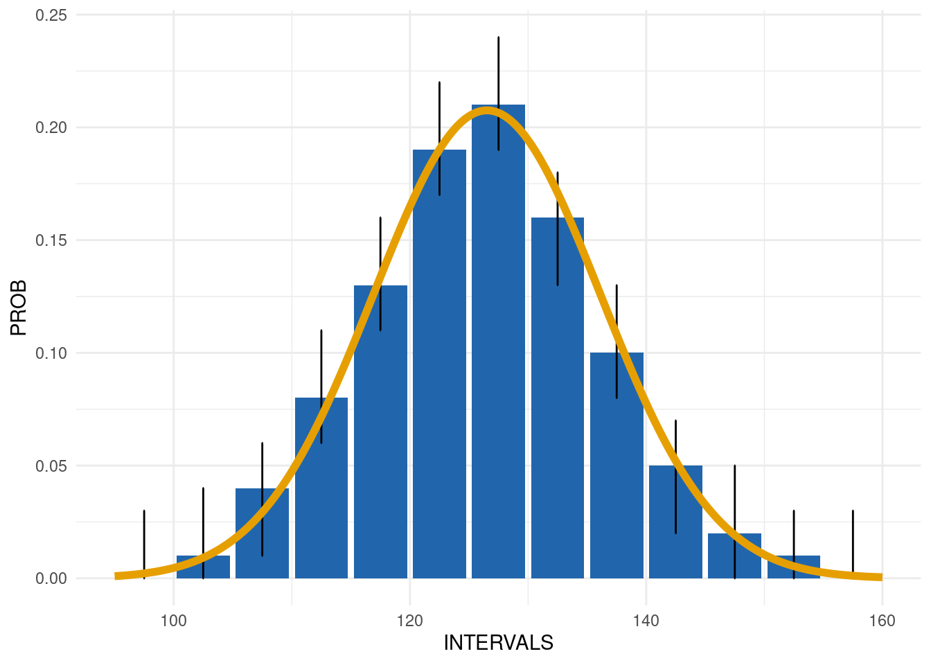
Output 3: Summary table
The third output, SummaryTable, is a table containing the response
variable and indicating whether the expected shape or scale is met
(GRADING = 0) or a deviation was found
(GRADING = 1). This table is necessary for the generic
function dataquieR::dq_report() to summarize all
information for the examined variables. Run
exp_dist_1$SummaryTable to see the output:
| Variables | FLG_acc_ud_shape |
|---|---|
| SBP_0 | 0 |
Example 2: uniform distributed data
This example inspects the shape or scale for the variable
GLOBAL_HEALTH_VAS_0 (Self-reported global health), which is
assumed to have a uniform distribution, and estimates the parameters of
its distribution (guess = TRUE):
exp_dist_2 <- acc_shape_or_scale(
  resp_vars = "GLOBAL_HEALTH_VAS_0",
  guess = TRUE,
  label_col = "LABEL",
  dist_col = "DISTRIBUTION",
  study_data = sd1,
  meta_data = md1
)
Output 1: Summary data
The output shows that the self-reported global health variable is
uniformly distributed (GRADING = 0):
exp_dist_2$SummaryData| INTERVALS | COUNT | PROB | EXP_PROB | EXP_COUNT | LOWER_CL | UPPER_CL | GRADING |
|---|---|---|---|---|---|---|---|
| 0.5 | 278 | 0.11 | 0.1 | 261.8 | 0.09 | 0.13 | 0 |
| 1.5 | 255 | 0.10 | 0.1 | 261.8 | 0.08 | 0.12 | 0 |
| 2.5 | 249 | 0.10 | 0.1 | 261.8 | 0.08 | 0.12 | 0 |
| 3.5 | 272 | 0.10 | 0.1 | 261.8 | 0.08 | 0.12 | 0 |
| 4.5 | 284 | 0.11 | 0.1 | 261.8 | 0.09 | 0.13 | 0 |
| 5.5 | 221 | 0.08 | 0.1 | 261.8 | 0.06 | 0.10 | 0 |
| 6.5 | 265 | 0.10 | 0.1 | 261.8 | 0.08 | 0.12 | 0 |
| 7.5 | 278 | 0.11 | 0.1 | 261.8 | 0.09 | 0.13 | 0 |
| 8.5 | 245 | 0.09 | 0.1 | 261.8 | 0.07 | 0.11 | 0 |
| 9.5 | 271 | 0.10 | 0.1 | 261.8 | 0.08 | 0.12 | 0 |
Output 2: Summary plot
The bar plot highlights in red the deviations from the uniform distribution (yellow line):
exp_dist_2$SummaryPlot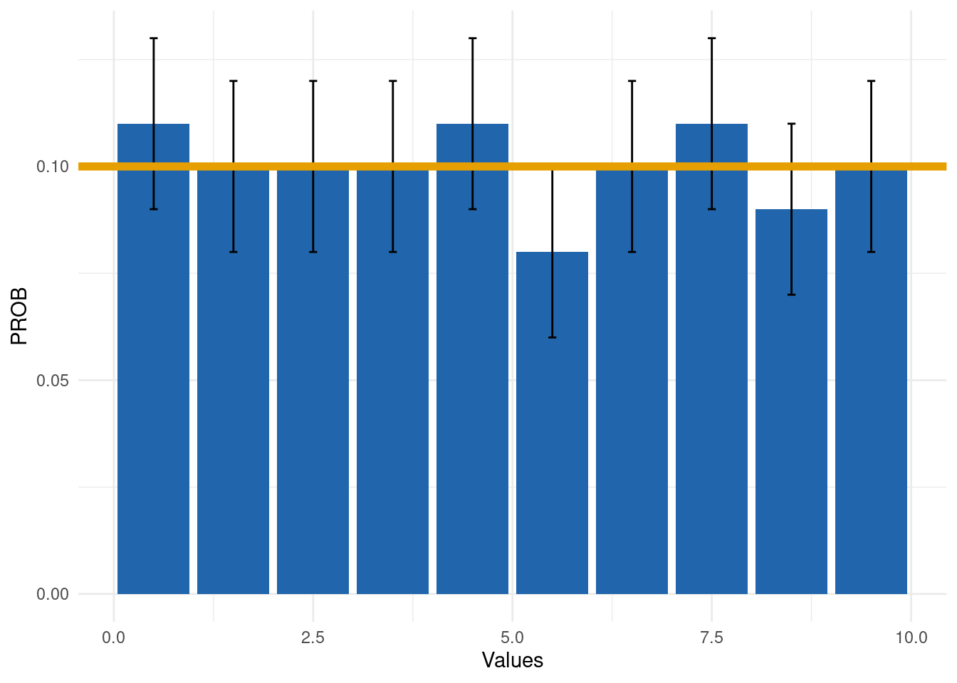
Example 3: gamma distributed data
The last example examines the variable CRP_0 (C-reactive
protein), which is assumed to have a gamma distribution, and estimates
the parameters of its distribution (guess = TRUE):
exp_dist_3 <- acc_shape_or_scale(
  resp_vars = "CRP_0",
  guess = TRUE,
  label_col = "LABEL",
  dist_col = "DISTRIBUTION",
  study_data = sd1,
  meta_data = md1
)
Output 1: Summary data frame
The result shows that the C-reactive protein is not uniformly
distributed (GRADING = 1 for the first interval):
exp_dist_3$SummaryData| INTERVALS | COUNT | PROB | EXP_PROB | EXP_COUNT | LOWER_CL | UPPER_CL | GRADING |
|---|---|---|---|---|---|---|---|
| 0.5 | 330 | 0.12 | 0.16 | 393.89 | 0.10 | 0.15 | 1 |
| 1.5 | 627 | 0.23 | 0.26 | 678.11 | 0.21 | 0.26 | 0 |
| 2.5 | 653 | 0.24 | 0.22 | 582.83 | 0.22 | 0.27 | 0 |
| 3.5 | 458 | 0.17 | 0.15 | 410.88 | 0.14 | 0.20 | 0 |
| 4.5 | 306 | 0.11 | 0.10 | 263.31 | 0.09 | 0.14 | 0 |
| 5.5 | 160 | 0.06 | 0.06 | 159.50 | 0.03 | 0.08 | 0 |
| 6.5 | 83 | 0.03 | 0.03 | 93.09 | 0.01 | 0.06 | 0 |
| 7.5 | 48 | 0.02 | 0.02 | 52.92 | 0.00 | 0.04 | 0 |
| 8.5 | 20 | 0.01 | 0.01 | 29.49 | 0.00 | 0.03 | 0 |
| 9.5 | 6 | 0.00 | 0.01 | 16.19 | 0.00 | 0.03 | 0 |
| 10.5 | 5 | 0.00 | 0.00 | 8.78 | 0.00 | 0.03 | 0 |
| 11.5 | 2 | 0.00 | 0.00 | 4.71 | 0.00 | 0.03 | 0 |
| 12.5 | 1 | 0.00 | 0.00 | 2.51 | 0.00 | 0.03 | 0 |
Output 2: Summary plot
Deviations are also evident in the plot, where the intervals outside of the expected distributions are highlighted in red:
exp_dist_3$SummaryPlot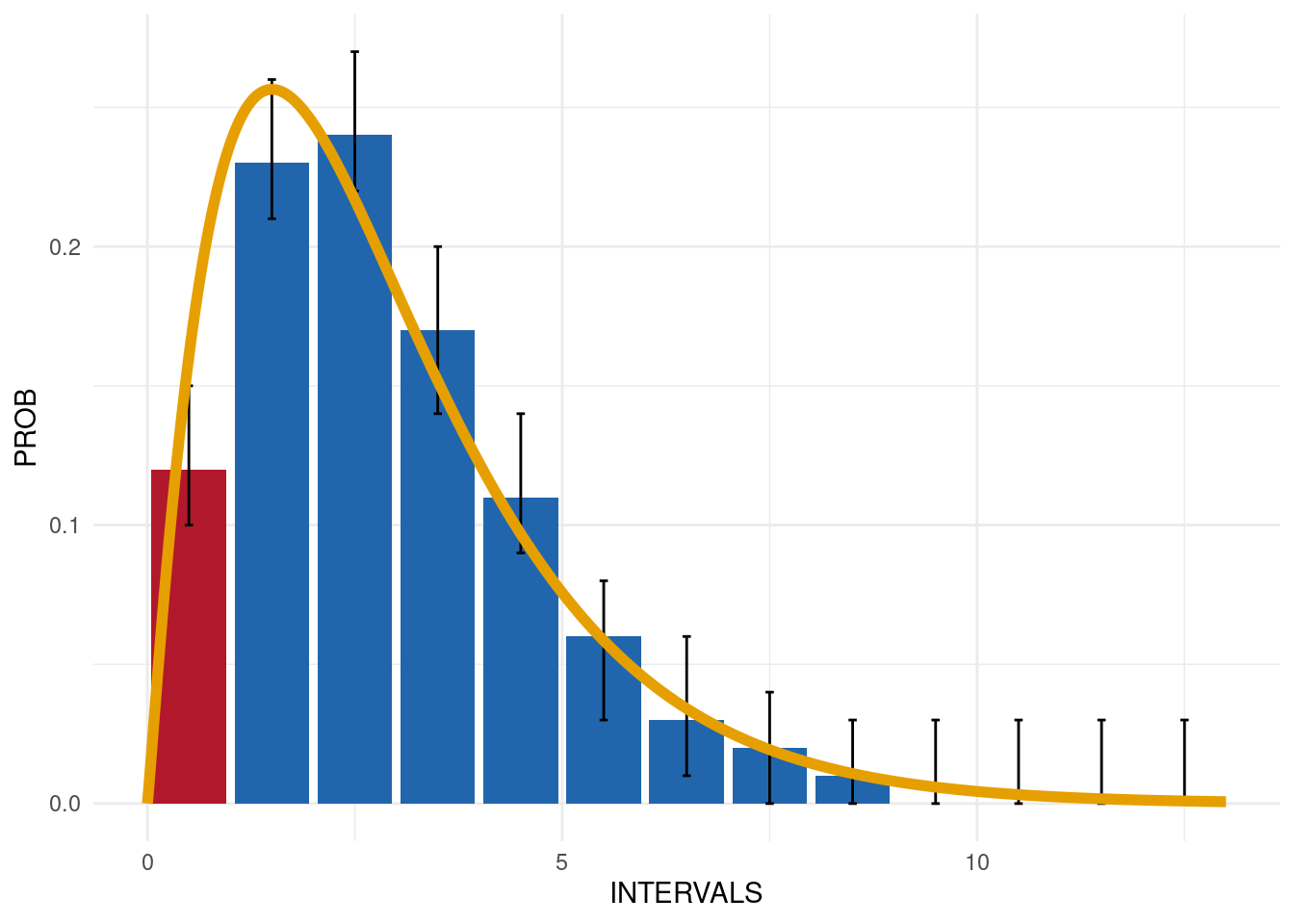
Interpretation
Any deviation from the distribution specified in the metadata is indicated in red.
Algorithm of the implementation
- This implementation is restricted to variables with float or integer data types.
- Remove missing codes from
resp_vars(if these are defined in the metadata).
- Extract the theoretical probability distribution from the metadata
(
normal,uniform, orgamma). - Estimate the distribution parameters if these are not specified by the user.
- Contrast the empirical versus the theoretical distribution in a histogram-like plot and in a summary data frame.
Limitations
Deviations from the empirical and theoretical distributions are frequent in real-world data. Applying statistical tests will create a considerable number of false-positives as consequence of multiple testing. Therefore, this implementation should not be used in an exploratory manner.
The acc_shape_or_scale function is currently restricted
to three classes of distributions (uniform, normal, and gamma). An
extension is planned for a future release.
Concept relations
- Data quality Indicator Unexpected scale
- Data quality Indicator Unexpected shape
